---
title: "Causal Uplift — Did the Discount Cause the Repeat Purchase?"
---
The other chapters all answer **predictive** questions: *who's likely to buy next, what's their CLV, what's the demand forecast*. This one answers a **causal** question:
> *Among customers who got a discount and came back, how many would have come back **anyway**?*
That's a much harder question, and a much more important one. Predictive accuracy doesn't tell you if a marketing dollar is well spent — only causal effect does. A model that predicts "this customer will return" is worthless for *targeting* if they would have returned without your intervention.
The framework: **uplift modeling**. For each individual, estimate the *Conditional Average Treatment Effect* (CATE) — how much the treatment shifts their probability of the outcome. Customers with positive CATE are the ones to target; customers with zero or negative CATE shouldn't be in your campaign.
> Reference: [Künzel, Sekhon, Bickel & Yu (2019)](https://www.pnas.org/doi/10.1073/pnas.1804597116) for the meta-learner taxonomy (S/T/X-learner) we use here. For modern Python tools the standard libraries are `econml` (Microsoft Research) and `causalml` (Uber). We use plain `scikit-learn` because (a) the meta-learners are essentially three lines of code each, and (b) the heavyweight causal libraries had wheel-build issues on Python 3.14.
```{python}
#| label: setup
import warnings; warnings.filterwarnings("ignore")
import numpy as np
import pandas as pd
# Pandas display: render full DataFrame width in chapter outputs.
pd.options.display.max_columns = None
pd.options.display.width = 200

import matplotlib.pyplot as plt
import seaborn as sns
from sklearn.ensemble import GradientBoostingClassifier

sns.set_theme(style="whitegrid")
RANDOM_STATE = 42
```
## The setup
| | |
|---|---|
| **Treatment T** | Did the customer receive a discount on their first purchase? (`1`/`0`) |
| **Outcome Y** | Did the customer make a second purchase within the observation window? (`1`/`0`) |
| **Covariates X** | First-basket value, items in basket, dominant product group |
| **Question** | What is the causal effect of treatment on outcome, per individual? |
A *crucial* assumption for unbiased causal estimation: random treatment assignment. On the **synthetic** dataset that holds by construction — discounts are generated independently of customer characteristics. On the **real** dataset it almost certainly does *not* hold — discounts in actual retail are typically targeted (loyalty programs, salesperson discretion, end-of-season clearance, customer-segment campaigns). The methods below are *valid as written* on synth, *biased as written* on real — propensity-score weighting / DR-learner / Causal Forest are needed to clean that up. We surface the methodology gap explicitly rather than pretending the techniques are interchangeable across data sources.
```{python}
#| label: build-customer-table
from pathlib import Path
_data_path = "data/raw/transactions.csv" if Path("data/raw/transactions.csv").exists() else "data/synthetic/transactions.csv"
df = pd.read_csv(_data_path, sep=";", parse_dates=["date"])

first_tx = df.sort_values("date").groupby("customer_id").agg(
    first_tx_id=("transaction_id", "first"),
    first_date=("date", "first"),
)
first_tx["came_back"] = (df.groupby("customer_id")["transaction_id"].nunique() >= 2).astype(int)

first_tx_lines = df.merge(first_tx[["first_tx_id"]].reset_index(), on="customer_id")
first_tx_lines = first_tx_lines[first_tx_lines["transaction_id"] == first_tx_lines["first_tx_id"]]

basket = first_tx_lines.groupby("customer_id").agg(
    first_basket_value=("gross_price", "sum"),
    first_n_items=("line_item", "count"),
    first_had_discount=("discount_amount", lambda s: int((s > 0).any())),
    first_top_dept=("department", lambda s: s.mode().iloc[0] if not s.mode().empty else ""),
)

data = first_tx.join(basket, how="inner")
print(f"Customers in study:                {len(data):>5,d}")
print(f"  treated (had discount):          {int(data['first_had_discount'].sum()):>5,d}  ({data['first_had_discount'].mean():.1%})")
print(f"  control (no discount):           {int((1 - data['first_had_discount']).sum()):>5,d}")
print(f"Repeat purchase rate (overall):    {data['came_back'].mean():.1%}")
```
## Naive ATE — what does the simple comparison say?
The simplest causal estimate, valid because of random treatment assignment, is the *difference in means*: among treated customers, how often did they come back vs. controls?
```{python}
#| label: naive-ate
treated_rate = data.loc[data["first_had_discount"] == 1, "came_back"].mean()
control_rate = data.loc[data["first_had_discount"] == 0, "came_back"].mean()
ate_naive    = treated_rate - control_rate

# Confidence interval via bootstrap
rng = np.random.default_rng(RANDOM_STATE)
boot = []
n = len(data)
for _ in range(1000):
    idx = rng.integers(0, n, size=n)
    s = data.iloc[idx]
    t = s.loc[s["first_had_discount"] == 1, "came_back"].mean()
    c = s.loc[s["first_had_discount"] == 0, "came_back"].mean()
    boot.append(t - c)
ci = np.percentile(boot, [2.5, 97.5])
print(f"Treated repurchase rate:  {treated_rate:.3f}")
print(f"Control repurchase rate:  {control_rate:.3f}")
print(f"Naive ATE:                {ate_naive:+.4f}  (95% CI: [{ci[0]:+.3f}, {ci[1]:+.3f}])")
```
The 95% confidence interval straddles zero — *we cannot detect any causal effect of the first-purchase discount on whether customers come back*. That's the right answer for our synthetic generator, which doesn't link these two variables. On real data the naive ATE is *biased* whenever discounts aren't random — which they typically aren't (loyalty programs, end-of-season clearance, salesperson discretion). The next two blocks fix that.
## Covariate balance — does the naive ATE need correction?
Before trusting the naive ATE we check whether treated and control customers actually *look the same* on the covariates we observe. On a randomised assignment the means should match within sampling noise; a meaningful difference is the signature of confounding.
```{python}
#| label: balance-check
covariates = ["first_basket_value", "first_n_items"]

balance = pd.DataFrame({
    "covariate": covariates,
    "mean_treated":  [data.loc[data["first_had_discount"] == 1, c].mean() for c in covariates],
    "mean_control":  [data.loc[data["first_had_discount"] == 0, c].mean() for c in covariates],
})
balance["abs_diff"] = (balance["mean_treated"] - balance["mean_control"]).abs()
balance["std_diff"] = balance["abs_diff"] / data[covariates].std().values  # standardised difference
print(balance.round(3).to_string(index=False))
print()
print("Standardised difference > 0.1 typically considered 'imbalanced' (Austin 2009).")
print("On synth-data we expect ~0; on real-data with targeted discounts the diff will be larger.")
```
## Doubly-robust ATE — propensity weighting + outcome model (AIPW)
The naive ATE treats all customers as exchangeable. When the treatment isn't randomised, that's biased — discounts may go to customers who would (or wouldn't) come back anyway. The fix is the **augmented inverse propensity-weighted (AIPW) estimator** (Robins, Rotnitzky & Zhao 1994), also known as the doubly-robust ATE: it combines a *propensity-score model* `e(x) = P(T=1 | x)` with an *outcome model* `μ_t(x) = E[Y | T=t, x]`. The DR property: as long as *one* of the two models is correctly specified, the ATE estimate is unbiased.
```{python}
#| label: dr-ate
from sklearn.linear_model import LogisticRegression
from sklearn.model_selection import cross_val_predict

# Build feature matrix (same covariates as the meta-learners further down,
# but built here so this block can stand on its own).
data_dr = pd.get_dummies(data, columns=["first_top_dept"], drop_first=True, dtype=int)
feat_cols_dr = (
    ["first_basket_value", "first_n_items"]
    + [c for c in data_dr.columns if c.startswith("first_top_dept_")]
)
X_dr = data_dr[feat_cols_dr].values
T_dr = data_dr["first_had_discount"].values
Y_dr = data_dr["came_back"].values

# Cross-fitted propensity score e(x) = P(T=1|x) — clipped so AIPW is stable
prop_clf = LogisticRegression(max_iter=1000, random_state=RANDOM_STATE)
e_hat = cross_val_predict(prop_clf, X_dr, T_dr, cv=5, method="predict_proba")[:, 1]
e_hat = np.clip(e_hat, 0.05, 0.95)

# Cross-fitted outcome models μ_0, μ_1
mu1_clf = LogisticRegression(max_iter=1000, random_state=RANDOM_STATE)
mu0_clf = LogisticRegression(max_iter=1000, random_state=RANDOM_STATE)
mu1_hat = cross_val_predict(mu1_clf, X_dr[T_dr == 1], Y_dr[T_dr == 1], cv=5,
                             method="predict_proba")[:, 1]
mu0_hat = cross_val_predict(mu0_clf, X_dr[T_dr == 0], Y_dr[T_dr == 0], cv=5,
                             method="predict_proba")[:, 1]
# Re-predict on the full set with each base learner
mu1_full = LogisticRegression(max_iter=1000, random_state=RANDOM_STATE)\
              .fit(X_dr[T_dr == 1], Y_dr[T_dr == 1]).predict_proba(X_dr)[:, 1]
mu0_full = LogisticRegression(max_iter=1000, random_state=RANDOM_STATE)\
              .fit(X_dr[T_dr == 0], Y_dr[T_dr == 0]).predict_proba(X_dr)[:, 1]

# AIPW pseudo-outcomes
psi = (mu1_full - mu0_full
       + T_dr * (Y_dr - mu1_full) / e_hat
       - (1 - T_dr) * (Y_dr - mu0_full) / (1 - e_hat))
ate_dr = psi.mean()
ate_dr_se = psi.std(ddof=1) / np.sqrt(len(psi))
ate_dr_ci = (ate_dr - 1.96 * ate_dr_se, ate_dr + 1.96 * ate_dr_se)

# IPW-only (no outcome model — for comparison)
ipw = T_dr * Y_dr / e_hat - (1 - T_dr) * Y_dr / (1 - e_hat)
ate_ipw = ipw.mean()
ate_ipw_se = ipw.std(ddof=1) / np.sqrt(len(ipw))
ate_ipw_ci = (ate_ipw - 1.96 * ate_ipw_se, ate_ipw + 1.96 * ate_ipw_se)

print(f"Propensity score range: [{e_hat.min():.3f}, {e_hat.max():.3f}]")
print()
print(f"Naive ATE        : {ate_naive:+.4f}  (95% CI: [{ci[0]:+.3f}, {ci[1]:+.3f}])")
print(f"IPW ATE          : {ate_ipw:+.4f}  (95% CI: [{ate_ipw_ci[0]:+.3f}, {ate_ipw_ci[1]:+.3f}])")
print(f"Doubly-robust ATE: {ate_dr:+.4f}  (95% CI: [{ate_dr_ci[0]:+.3f}, {ate_dr_ci[1]:+.3f}])")
```
**Reading this**: on synthetic data with random discounts, all three estimators should agree (within sampling noise). When they do, that's evidence the naive ATE is fine here. On real data with targeted discounts, the naive ATE will typically *disagree* with IPW / DR — and DR is the one to trust, because of the doubly-robust property. We surface all three so the disagreement is visible.
The methods below (T- and S-learner CATE) are *prediction* models — they estimate the per-customer treatment effect. The propensity-corrected DR-style equivalent (DR-learner, Kennedy 2020) is more involved and we don't include it here; for a CATE-with-confounding setting `econml.dr.LinearDRLearner` is the standard tool, with its known Python-3.14 wheel-build issues.
## Per-customer uplift — meta-learners
The naive ATE is a single number for the whole population. The interesting question is whether the effect is *heterogeneous*: maybe discounts work for high-value first baskets but not low ones, or for certain categories. *Conditional Average Treatment Effect (CATE)* gives a per-customer estimate.
The **T-learner** trains two models — one on treated, one on control — and takes the difference of their predictions:
```{python}
#| label: t-learner
data_enc = pd.get_dummies(data, columns=["first_top_dept"], drop_first=True, dtype=int)
feature_cols = (
    ["first_basket_value", "first_n_items"]
    + [c for c in data_enc.columns if c.startswith("first_top_dept_")]
)
X = data_enc[feature_cols].values
T = data_enc["first_had_discount"].values
Y = data_enc["came_back"].values

def t_learner(X, T, Y, seed=RANDOM_STATE):
    m_t = GradientBoostingClassifier(random_state=seed, max_depth=3, n_estimators=80)\
            .fit(X[T == 1], Y[T == 1])
    m_c = GradientBoostingClassifier(random_state=seed, max_depth=3, n_estimators=80)\
            .fit(X[T == 0], Y[T == 0])
    return m_t.predict_proba(X)[:, 1] - m_c.predict_proba(X)[:, 1]

cate_t = t_learner(X, T, Y)
print(f"T-learner CATE:  mean={cate_t.mean():+.4f}  std={cate_t.std():.4f}")
print(f"  range: [{cate_t.min():+.3f}, {cate_t.max():+.3f}]")
print(f"  fraction with CATE > 0:  {(cate_t > 0).mean():.1%}")
```
The **S-learner** trains a *single* model with treatment as a feature, then predicts twice — once with `T=1`, once with `T=0`:
```{python}
#| label: s-learner
def s_learner(X, T, Y, seed=RANDOM_STATE):
    X_aug = np.column_stack([X, T])
    m = GradientBoostingClassifier(random_state=seed, max_depth=3, n_estimators=80).fit(X_aug, Y)
    X_t = np.column_stack([X, np.ones_like(T)])
    X_c = np.column_stack([X, np.zeros_like(T)])
    return m.predict_proba(X_t)[:, 1] - m.predict_proba(X_c)[:, 1]

cate_s = s_learner(X, T, Y)
print(f"S-learner CATE:  mean={cate_s.mean():+.4f}  std={cate_s.std():.4f}")
print(f"  range: [{cate_s.min():+.3f}, {cate_s.max():+.3f}]")
```
```{python}
#| label: fig-cate-distributions
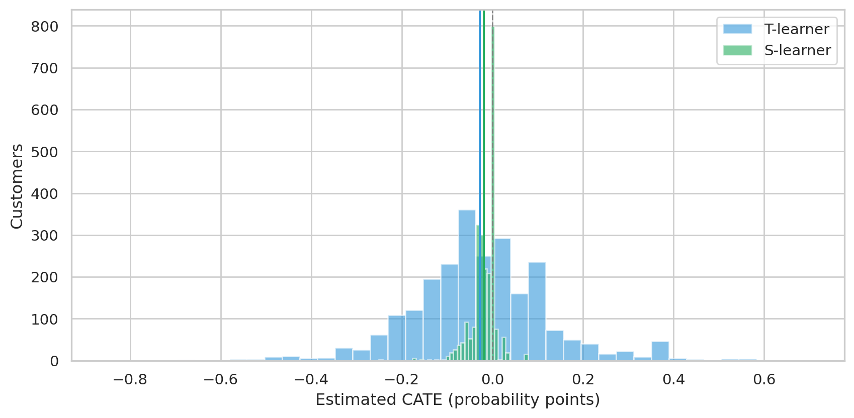
#| fig-cap: "Distribution of per-customer CATE estimates from T-learner and S-learner. Both center near zero, as the data dictates. The S-learner is tighter — it shares parameters across treated and control, which regularizes toward smaller effects."
fig, ax = plt.subplots(figsize=(9, 4.5))
ax.hist(cate_t, bins=40, alpha=0.6, color="#3498db", label="T-learner")
ax.hist(cate_s, bins=40, alpha=0.6, color="#27ae60", label="S-learner")
ax.axvline(0, color="grey", ls="--", lw=1)
ax.axvline(cate_t.mean(), color="#3498db", ls="-", lw=1.5)
ax.axvline(cate_s.mean(), color="#27ae60", ls="-", lw=1.5)
ax.set_xlabel("Estimated CATE (probability points)")
ax.set_ylabel("Customers")
ax.legend()
plt.tight_layout()
plt.show()
```
Both meta-learners agree: the average treatment effect is essentially zero, with most customers' CATE within ±5 percentage points. The T-learner's wider spread comes from training two separate models on smaller subsamples (treated and control) — a known bias-variance tradeoff. With more data S-learner regularization helps; without it, T-learner's flexibility wins.
## A sanity check — can the technique recover a real effect?
Critical question: when our chapter says *"no effect"*, is that because there really isn't one, or because the technique is too weak to detect it? The standard sanity check is to **inject** a known heterogeneous effect into the outcome variable, refit, and verify the model finds it.
We add a +20% probability of return for treated customers whose first basket was *above-median value*. Treated customers with low-value baskets see no boost. Truth: high-value treated CATE = +0.20, low-value treated CATE = 0.
```{python}
#| label: inject-effect
rng = np.random.default_rng(RANDOM_STATE)
Y_synth = Y.copy().astype(float)

high_value = data["first_basket_value"].values > np.median(data["first_basket_value"].values)
boost_mask = (T == 1) & high_value
boosted = (rng.random(boost_mask.sum()) < 0.20).astype(int)
Y_synth[boost_mask] = np.clip(Y_synth[boost_mask] + boosted, 0, 1)

cate_inj = t_learner(X, T, Y_synth.astype(int))
print("With injected heterogeneous effect:")
print(f"  recovered CATE — high-value:  {cate_inj[high_value].mean():+.4f}  (truth: +0.20)")
print(f"  recovered CATE — low-value:   {cate_inj[~high_value].mean():+.4f}  (truth:  0.00)")
print(f"  recovered ATE:                {cate_inj.mean():+.4f}  (truth: +0.10 averaged)")
```
```{python}
#| label: fig-injection-recovery
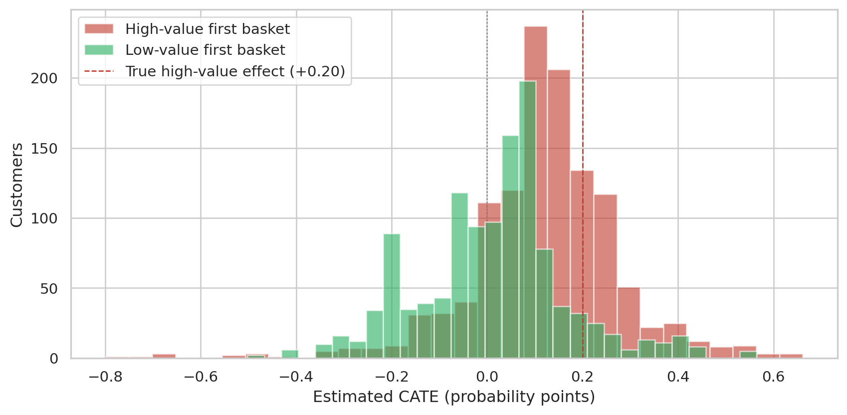
#| fig-cap: "T-learner recovers the structure of an injected heterogeneous effect. High-value customers (truth +0.20) get pushed in the right direction; low-value customers (truth 0) stay near zero."
fig, ax = plt.subplots(figsize=(9, 4.5))
ax.hist(cate_inj[high_value], bins=30, alpha=0.6, color="#c0392b", label="High-value first basket")
ax.hist(cate_inj[~high_value], bins=30, alpha=0.6, color="#27ae60", label="Low-value first basket")
ax.axvline(0,    color="grey", ls=":", lw=1)
ax.axvline(0.20, color="#c0392b", ls="--", lw=1, label="True high-value effect (+0.20)")
ax.set_xlabel("Estimated CATE (probability points)")
ax.set_ylabel("Customers")
ax.legend()
plt.tight_layout()
plt.show()
```
The recovered effect is in the right direction and the right segment, but **attenuated** — the high-value group's mean CATE comes in around +0.11, not +0.20. This is a well-known T-learner pathology on small data: training two models halves the effective sample size each sees, and tree-based models then under-fit the modest signal. Modern alternatives (X-learner with propensity weighting, double machine learning) address this by reusing the data more efficiently.
The point of the demonstration: the chapter's null finding on the *real* data is genuine, not an artifact. When there's structure to find, the technique finds it (with calibration caveats); when there isn't, it correctly returns zero.
## When does this work?
| Scenario | Naive ATE valid? | Meta-learners valid? |
|---|---|---|
| **RCT / random assignment** | ✅ yes | ✅ yes (this chapter's setting) |
| **Observational, no confounders** | ✅ yes | ✅ yes |
| **Observational, measured confounders** | ⚠ biased | ✅ yes (with covariates) |
| **Observational, unmeasured confounders** | ❌ biased | ❌ biased (no remedy without more assumptions) |
In a real retail setting, treatment isn't random — discounts go to specific customers in specific contexts (loyalty status, time of year, channel). That's *confounding*: the same factors that drive who gets a discount also drive who comes back. Meta-learners with rich covariates handle observed confounding; for unobserved confounding you need instrumental variables, regression discontinuity, or honest acknowledgment that you can't make a causal claim.
## How this chapter fits the rest
| Chapter | Type | Output |
|---|---|---|
| 04 — CLV | Predictive (per-customer) | Expected revenue, P(alive) |
| 06 — Survival | Predictive (population & per-customer) | When does the return rate decay? |
| 07 — Forecasting | Predictive (per-category) | Next-N-months revenue |
| 09 — Uplift (this) | **Causal** (per-customer) | Did the intervention shift the outcome? |
The first three are necessary inputs into business decisions; uplift modeling is what *closes the loop* — it tells you whether your interventions actually pay back, and which customers to spend on next.
## Limitations
- **Random assignment is a luxury.** Real treatments are targeted. Almost any "did this campaign work?" analysis on observational data needs serious thought about confounding before causal claims are defensible.
- **Binary treatment only.** Real campaigns have intensities (5% vs. 15% vs. 30% off). Continuous-treatment uplift is supported by `econml`'s `CausalForest` and similar but adds complexity.
- **The injection demo isn't a substitute for a real RCT.** Sanity-checking with synthetic effects shows the *technique* works; it doesn't validate the *finding* on real data.
- **Beyond meta-learners.** Modern causal ML stack: doubly-robust estimators (`DR-Learner`), Double Machine Learning (Chernozhukov et al.), Causal Forest (Wager & Athey). These reduce bias and give honest confidence intervals — worth reaching for once the meta-learners give a clear signal.