Survival Analysis — Time to First Repeat Purchase

The CLV chapter answered whether a customer comes back, with what probability and what value. This chapter answers a sharper question: when?

Specifically: among customers who made one purchase, how does the probability of a second purchase decay over time? At what point does the residual hope of a return drop low enough that we should either trigger a win-back campaign or write the customer off?

Survival analysis is the right tool because the data is right-censored: many customers we observe haven’t returned yet — but might. Treating “hasn’t come back” as “won’t come back” would massively overstate churn. Survival analysis handles censoring as a first-class concept.

Reference: Klein & Moeschberger (2003) is the standard text. Implementation via the lifelines Python package — same ecosystem as the lifetimes package used in chapter 04.

Code

import numpy as np
import pandas as pd
import matplotlib.pyplot as plt
import seaborn as sns
from lifelines import KaplanMeierFitter, CoxPHFitter
from lifelines.statistics import multivariate_logrank_test

sns.set_theme(style="whitegrid")
RANK_PALETTE = ["#27ae60", "#3498db", "#f39c12", "#c0392b"]

Defining the survival event

For each customer we need three things:

Quantity	Definition
`duration`	Days from first purchase to either (a) their second purchase, or (b) the observation end if they haven’t returned
`event`	`1` if they made a second purchase within the observation window, `0` otherwise (censored)
`T`	Days they’ve been observed since their first purchase — used to gauge how much information we have

The censoring distinction is critical: a customer who first bought 700 days ago and never returned is very different from one who bought 7 days ago and hasn’t (yet) returned. The first is a probable churn; the second is an unknown.

Code

from pathlib import Path
_data_path = "data/raw/transactions.csv" if Path("data/raw/transactions.csv").exists() else "data/synthetic/transactions.csv"
df = pd.read_csv(_data_path, sep=";", parse_dates=["date"])

tx = df.groupby(["customer_id", "transaction_id", "date"], as_index=False)["gross_price"].sum()
OBS_END = tx["date"].max()

ranked = tx.sort_values(["customer_id", "date"]).copy()
ranked["rank"] = ranked.groupby("customer_id").cumcount()
first  = ranked[ranked["rank"] == 0].set_index("customer_id")[["date", "gross_price"]]\
            .rename(columns={"date": "first_date", "gross_price": "first_value"})
second = ranked[ranked["rank"] == 1].set_index("customer_id")[["date"]]\
            .rename(columns={"date": "second_date"})

surv = first.join(second, how="left")
surv["event"] = surv["second_date"].notna().astype(int)
surv["duration"] = np.where(
    surv["event"] == 1,
    (surv["second_date"] - surv["first_date"]).dt.days,
    (OBS_END - surv["first_date"]).dt.days,
)
surv = surv[surv["duration"] > 0].copy()

print(f"Customers in cohort:        {len(surv):>5,d}")
print(f"  observed second purchase: {int(surv['event'].sum()):>5,d}  ({surv['event'].mean():.1%})")
print(f"  censored at OBS_END:      {int((surv['event'] == 0).sum()):>5,d}  ({1 - surv['event'].mean():.1%})")
print(f"Duration range: {int(surv['duration'].min())}–{int(surv['duration'].max())} days")

Customers in cohort:        2,400
  observed second purchase:   692  (28.8%)
  censored at OBS_END:      1,708  (71.2%)
Duration range: 1–730 days

Roughly 29% of customers in the cohort returned within the observation window. The remaining 71% are censored — some genuinely never will return, others simply haven’t had enough time yet.

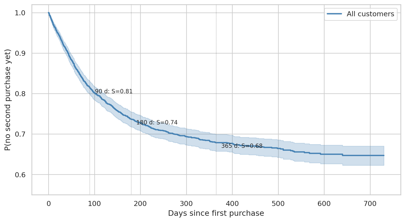
Population survival curve — Kaplan-Meier

The Kaplan-Meier estimator gives a non-parametric estimate of the probability that a customer has not returned by time t. It’s a step function that drops at each observed second purchase, weighted to account for censoring.

Code

kmf = KaplanMeierFitter()
kmf.fit(surv["duration"], surv["event"], label="All customers")

fig, ax = plt.subplots(figsize=(9, 5))
kmf.plot_survival_function(ax=ax, color="steelblue", lw=2, ci_show=True)
for d, label in [(90, "90 d"), (180, "180 d"), (365, "365 d")]:
    s = float(kmf.survival_function_at_times(d).iloc[0])
    ax.axvline(d, color="grey", ls=":", lw=0.7)
    ax.annotate(f"{label}: S={s:.2f}", (d, s), xytext=(8, -8),
                textcoords="offset points", fontsize=9)
ax.set_xlabel("Days since first purchase")
ax.set_ylabel("P(no second purchase yet)")
ax.set_ylim(0.55, 1.02)
ax.legend()
plt.tight_layout()
plt.show()

Figure 1: Population survival: probability that a first-time buyer has not yet made a second purchase by day t. The horizontal lines mark the 90/180/365-day milestones.

Reading the curve:

After 90 days, ~81% of first-time buyers still haven’t come back. This isn’t alarming — the “win-back” zone is much later.
By 180 days, ~74% remain non-repeat. Half a year of silence is meaningful but not yet final.
By 365 days, the curve has flattened to ~68%. The tail of customers who will eventually return after a year is small.

The fact that the curve doesn’t decay to zero (median survival is ∞) reflects a real-retail truth: the majority of one-time buyers stay one-time buyers. Survival analysis quantifies which fraction and when, instead of pretending everyone returns.

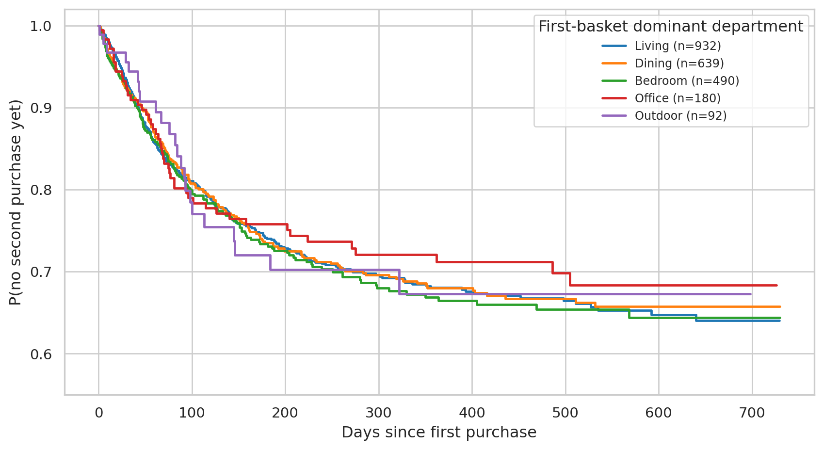
Stratification — does the first basket predict return rate?

Beyond the population, we want to know if first-purchase characteristics shift the curve. Cohort by the department of the first basket — six store-floor sections is the right level of granularity for a covariate (more levels mean noisier coefficients, fewer mean less interpretable):

Code

first_tx_id = df.sort_values("date").groupby("customer_id")["transaction_id"].first()
first_tx_lines = df.merge(
    first_tx_id.rename("first_tx_id").reset_index(),
    on="customer_id",
).query("transaction_id == first_tx_id")

basket_features = first_tx_lines.groupby("customer_id").agg(
    first_basket_value=("gross_price", "sum"),
    first_n_items=("line_item", "count"),
    first_top_dept=("department", lambda s: s.mode().iloc[0] if not s.mode().empty else ""),
    first_had_discount=("discount_amount", lambda s: (s > 0).any()),
)

surv_full = surv.join(basket_features, how="left")
surv_full["first_had_discount"] = surv_full["first_had_discount"].astype(int)
surv_full[["duration", "event", "first_basket_value", "first_n_items",
           "first_top_dept", "first_had_discount"]].describe(include="all").round(2)

	duration	event	first_basket_value	first_n_items	first_top_dept	first_had_discount
count	2400.00	2400.00	2400.00	2400.00	2400	2400.00
unique	NaN	NaN	NaN	NaN	6	NaN
top	NaN	NaN	NaN	NaN	Living	NaN
freq	NaN	NaN	NaN	NaN	932	NaN
mean	277.79	0.29	736.17	1.83	NaN	0.25
std	220.17	0.45	751.60	1.09	NaN	0.43
min	1.00	0.00	18.06	1.00	NaN	0.00
25%	76.00	0.00	163.55	1.00	NaN	0.00
50%	223.50	0.00	418.69	1.00	NaN	0.00
75%	456.25	1.00	1139.89	2.00	NaN	0.00
max	730.00	1.00	4091.98	6.00	NaN	1.00

Code

top_groups = surv_full["first_top_dept"].value_counts().head(5).index.tolist()

fig, ax = plt.subplots(figsize=(9, 5))
palette = sns.color_palette("tab10", n_colors=len(top_groups))
for g, c in zip(top_groups, palette):
    mask = surv_full["first_top_dept"] == g
    n = int(mask.sum())
    KaplanMeierFitter().fit(
        surv_full.loc[mask, "duration"], surv_full.loc[mask, "event"], label=f"{g} (n={n})"
    ).plot_survival_function(ax=ax, color=c, ci_show=False, lw=1.8)

ax.set_xlabel("Days since first purchase")
ax.set_ylabel("P(no second purchase yet)")
ax.set_ylim(0.55, 1.02)
ax.legend(title="First-basket dominant department", fontsize=9)
plt.tight_layout()
plt.show()

Figure 2: Survival curves stratified by the first basket’s dominant department. Overlapping curves and confidence intervals = no real differences between groups.

Code

result = multivariate_logrank_test(
    surv_full["duration"], surv_full["first_top_dept"], surv_full["event"],
)
print(f"Multivariate log-rank test across departments:")
print(f"  test statistic:  {result.test_statistic:.2f}")
print(f"  p-value:         {result.p_value:.4f}")

Multivariate log-rank test across departments:
  test statistic:  2.26
  p-value:         0.8114

If the curves were materially different, we’d see clear separation and a small p-value. Here they sit on top of one another and the log-rank test fails to reject the null — the first basket’s department does not predict the return timing in this dataset.

That’s not a bug; it’s the right answer. We engineered customer behavior to be independent of what they bought first (lifetime and rate are random per customer, not conditioned on basket contents). A real dataset would almost certainly show category effects — but inventing them here would be cheating.

Cox proportional hazards — multiple covariates

A Cox PH model estimates how a unit increase in each covariate multiplies the hazard (instantaneous rate of return). Hazard ratio > 1 = covariate accelerates return; < 1 = covariate delays it.

Code

cph_data = surv_full.dropna(subset=["first_basket_value"]).copy()
cph_data["log_first_value"] = np.log1p(cph_data["first_basket_value"])
cph_data = pd.get_dummies(cph_data, columns=["first_top_dept"], drop_first=True, dtype=int)

feature_cols = (
    ["log_first_value", "first_n_items", "first_had_discount"]
    + [c for c in cph_data.columns if c.startswith("first_top_dept_")]
)
cph_input = cph_data[["duration", "event"] + feature_cols].dropna()

cph = CoxPHFitter(penalizer=0.01)
cph.fit(cph_input, duration_col="duration", event_col="event")
cph.summary[["coef", "exp(coef)", "exp(coef) lower 95%", "exp(coef) upper 95%", "p"]].round(3)

	coef	exp(coef)	exp(coef) lower 95%	exp(coef) upper 95%	p
covariate
log_first_value	-0.010	0.990	0.909	1.079	0.820
first_n_items	0.065	1.068	0.973	1.171	0.166
first_had_discount	-0.096	0.909	0.759	1.088	0.298
first_top_dept_Dining	-0.038	0.963	0.778	1.190	0.725
first_top_dept_Living	-0.004	0.996	0.814	1.219	0.969
first_top_dept_Office	-0.106	0.899	0.655	1.233	0.509
first_top_dept_Outdoor	-0.022	0.978	0.633	1.512	0.922
first_top_dept_Storage	0.284	1.328	0.856	2.060	0.206

Reading the summary table:

exp(coef) is the hazard ratio. Values near 1.0 mean no detectable effect.
p column tells us whether the effect is statistically distinguishable from no effect.

For this synthetic dataset, all coefficients are near 1.0 with high p-values — the conclusion the model honestly gives us is “the first-purchase characteristics we measured do not predict when customers return.” This is the right read of the data.

In a real retail setting you’d typically expect some non-trivial effects:

Higher first-basket value → slightly higher hazard (engaged customers buy more often)
First purchase included a discount → variable; sometimes discount-sensitive shoppers churn faster
Specific product categories → durables (furniture) vs. consumables (decor) have very different repurchase tempos

The chapter machinery transfers directly when those effects are present.

Practical translation

Even with no covariate effects, the population survival curve gives concrete numbers for retention operations:

Code

for d in [30, 60, 90, 180, 270, 365, 540]:
    s = float(kmf.survival_function_at_times(d).iloc[0])
    print(f"  {d:>4d} days silent → {1-s:.1%} of cohort has returned by now, "
          f"{s:.1%} still pending")

    30 days silent → 7.4% of cohort has returned by now, 92.6% still pending
    60 days silent → 13.9% of cohort has returned by now, 86.1% still pending
    90 days silent → 18.6% of cohort has returned by now, 81.4% still pending
   180 days silent → 26.3% of cohort has returned by now, 73.7% still pending
   270 days silent → 29.9% of cohort has returned by now, 70.1% still pending
   365 days silent → 32.1% of cohort has returned by now, 67.9% still pending
   540 days silent → 34.4% of cohort has returned by now, 65.6% still pending

A defensible operational rule:

Day 1–90: silence is normal; do nothing automated. Most repeat-buyers don’t yet show up.
Day 90–180: customer is in the “warm-but-quiet” zone — a soft re-engagement (newsletter, product update) is appropriate.
Day 180–365: half the eventual returners come back in this window. A targeted discount or recommendation email is the highest-leverage intervention here.
Day 365+: curve has largely flattened. Most who haven’t come back by now won’t. Either invest heavily (reactivation campaign with a meaningful offer) or accept the loss and stop spending.

How this chapter complements the others

Chapter	Question	Output
04 — CLV (BG/NBD)	Will this specific customer come back, and how much will they spend?	Per-customer P(alive), expected purchases, 12-month CLV
06 — Survival (this)	When does a customer’s return probability decay, and what speeds or slows it?	Population & stratified survival curves, hazard ratios, intervention thresholds

CLV is forward-looking, individual, monetary. Survival is time-aware, population, operational. Together they answer “who to spend on, and when to spend”.

Limitations

No effects in synthetic data. The covariate analysis is honest but unexciting — by construction, no first-purchase feature drives the return timing here. With real data, hazard ratios on category, price tier, and discount usage would typically all be non-null.
Right-censoring is heavy. 71% of the cohort is censored. The Kaplan-Meier estimator handles this correctly, but the precision of the tail of the curve degrades as fewer customers remain at risk.
First-to-second only. We only modeled time-to-first-repeat. A natural extension is recurrent-event survival: looking at all inter-purchase gaps. lifelines supports this via WeibullAFTFitter with frailty terms; it’s a follow-up worth doing if the data has enough repeat-buyers.