---
title: "Association Rules — Market Basket Analysis"
---
Given a pile of receipts, *association rule mining* discovers patterns of the form
*"customers who buy A and B also tend to buy C"*. The textbook algorithm is
[Apriori](https://en.wikipedia.org/wiki/Apriori_algorithm) — fast, deterministic, and the standard starting point.
A rule $A \Rightarrow B$ is characterized by three numbers:
- **Support** — fraction of baskets containing $A \cup B$, i.e. $P(A \cup B)$. High support = the rule covers a meaningful share of customers.
- **Confidence** — given $A$ in the basket, how likely is $B$, i.e. $P(B \mid A)$. High confidence = the rule is reliable.
- **Lift** — how much more often $B$ shows up when $A$ is present compared to its baseline rate, i.e. $\frac{P(B \mid A)}{P(B)}$. Lift > 1 = positive association.
We mine rules at minimum support 0.001 and minimum confidence 0.5, then sort by confidence. Two implementations run side by side: `arules` in R and `mlxtend` in Python.
## Data
For market basket analysis we only need two columns: the basket identifier (`transaction_id`) and the item identifier. We use `article_name`, not `article_id` — so a "sofa" rule isn't fragmented across three SKUs of the same product.
```{r}
#| label: load-data-r
library(dplyr)
library(readr)

.data_path <- if (file.exists("data/raw/transactions.csv")) "data/raw/transactions.csv" else "data/synthetic/transactions.csv"
raw <- read_delim(.data_path, delim = ";", show_col_types = FALSE)
cat("rows:", nrow(raw), "  baskets:", n_distinct(raw$transaction_id), "  items:", n_distinct(raw$article_name), "\n")
```
## R — `arules`
### Build the transaction object
```{r}
#| label: build-transactions
library(arules)
# C locale needed for stable sort of items across baskets; without it, real
# data with German characters (Kopfstütze, Eßtisch, …) hits a sparse-matrix
# invariant violation when arules constructs its internal indexing.
Sys.setlocale("LC_COLLATE", "C")
# Defensive: drop missing / empty article names before grouping. Real data
# typically has a long tail of unparseable rows (returns, miscoded items, ...);
# arules can't construct its sparse matrix if any items are NA.
clean <- raw[!is.na(raw$article_name) & nchar(trimws(raw$article_name)) > 0, ]
clean$article_name <- trimws(clean$article_name)

baskets <- split(clean$article_name, clean$transaction_id)
baskets <- lapply(baskets, function(b) sort(unique(b)))  # sort + dedupe
trans   <- as(baskets, "transactions")
summary(trans)
```
### Item frequency
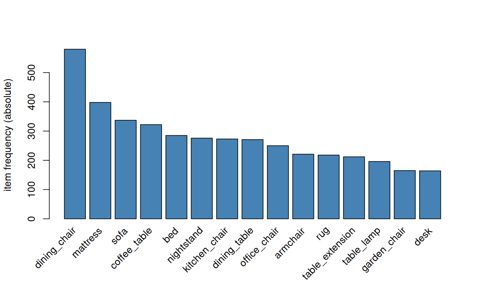
The 15 most-purchased products:
```{r}
#| label: fig-item-frequency
#| fig-cap: "Top 15 articles by basket appearance. On real data the top items are often *generic* names ('esstisch', 'stuhl') rather than model-specific labels — see the data-quality note below."
itemFrequencyPlot(trans, topN = 15, type = "absolute",
                  col = "steelblue", main = "")
```
The leading items reflect what the catalog stocks at scale — typically chairs (bought in sets of 2/4/6 around tables), table-extension components, and core upholstered/storage items.
**Data-quality note for the real-data render**: many of the dominant items in the chart are generic names — `esstisch`, `stuhl`, `eckgarnitur` — rather than model-specific labels (`esstisch ca 180 x 90 cm`, `esstisch cartago`). That's how the source system was filled in: salespeople often entered the basic Artikelbezeichnung and put model + size info into separate `Modell` / `Artikelnummer` fields. So the apparent concentration on a handful of generic items reflects how the catalogue was *recorded*, not how customers actually shopped — many distinct Cartago / Olivia / etc. variants sit underneath each generic label. Co-purchase rules at this level are still meaningful (chairs do go with tables, regardless of model), but model-level cross-sell ("Cartago-Esstisch zieht Cartago-Stuhl") is *not* what this view surfaces. For that you'd need to either pre-concatenate `article_name + model` (the `family_model` granularity from `docs/GRANULARITY_ANALYSIS.md`, ~5 300 items) or work at SKU level (`article_id`, ~3 500 items, used by chapter 08).
### Mining rules
```{r}
#| label: apriori-r
rules <- apriori(trans,
                 parameter = list(support = 0.001, confidence = 0.5),
                 control   = list(verbose = FALSE))
cat("Total rules found:", length(rules), "\n")
```
Apriori returns hundreds of rules at this threshold. Sorting by confidence puts the most reliable ones first — but the very top is dominated by *complex* rules of the form `{A, B, C, D} ⇒ E`. These are technically high-confidence (often 100%) but cover so few baskets that they're noisy.
A second source of clutter is **subsumption**: many rules are redundant restatements of stronger rules. `arules::is.redundant()` is the canonical filter — it removes a rule whenever a more general rule (a strict subset of its antecedent leading to the same consequent) has equal-or-better confidence. Standard Apriori-postprocessing since the early 2000s.
```{r}
#| label: redundancy-filter
non_redundant <- rules[!is.redundant(rules)]
cat("After arules::is.redundant() filter:",
    length(non_redundant), "of", length(rules), "rules remain\n")
```
The headline patterns are the **simple** rules: one item on the left, one on the right.
```{r}
#| label: simple-rules-r
simple <- subset(non_redundant, size(non_redundant) == 2)
simple_sorted <- sort(simple, by = "confidence", decreasing = TRUE)
inspect(head(simple_sorted, 10))
```
These are *all* simple rules sorted by confidence — including the definitional ones that aren't really insights. The Python section below adds richer interest measures (lift, conviction, leverage), substring-relation annotation, and **three separate views** on the same rule set — bundle composition, cross-sell, and top-insights — which is what stakeholders actually consume.
### What about the complex rules?
Multi-item rules can hit 100% confidence because they're highly specific — `{bed, mattress, table_extension} ⇒ dining_table` triggers only on the rare baskets where someone happens to buy bedroom and dining furniture together. They're not noise, but they're more interesting as patterns to investigate than as rules to act on.
### Visualizing rules
```{r}
#| label: fig-rules-scatter
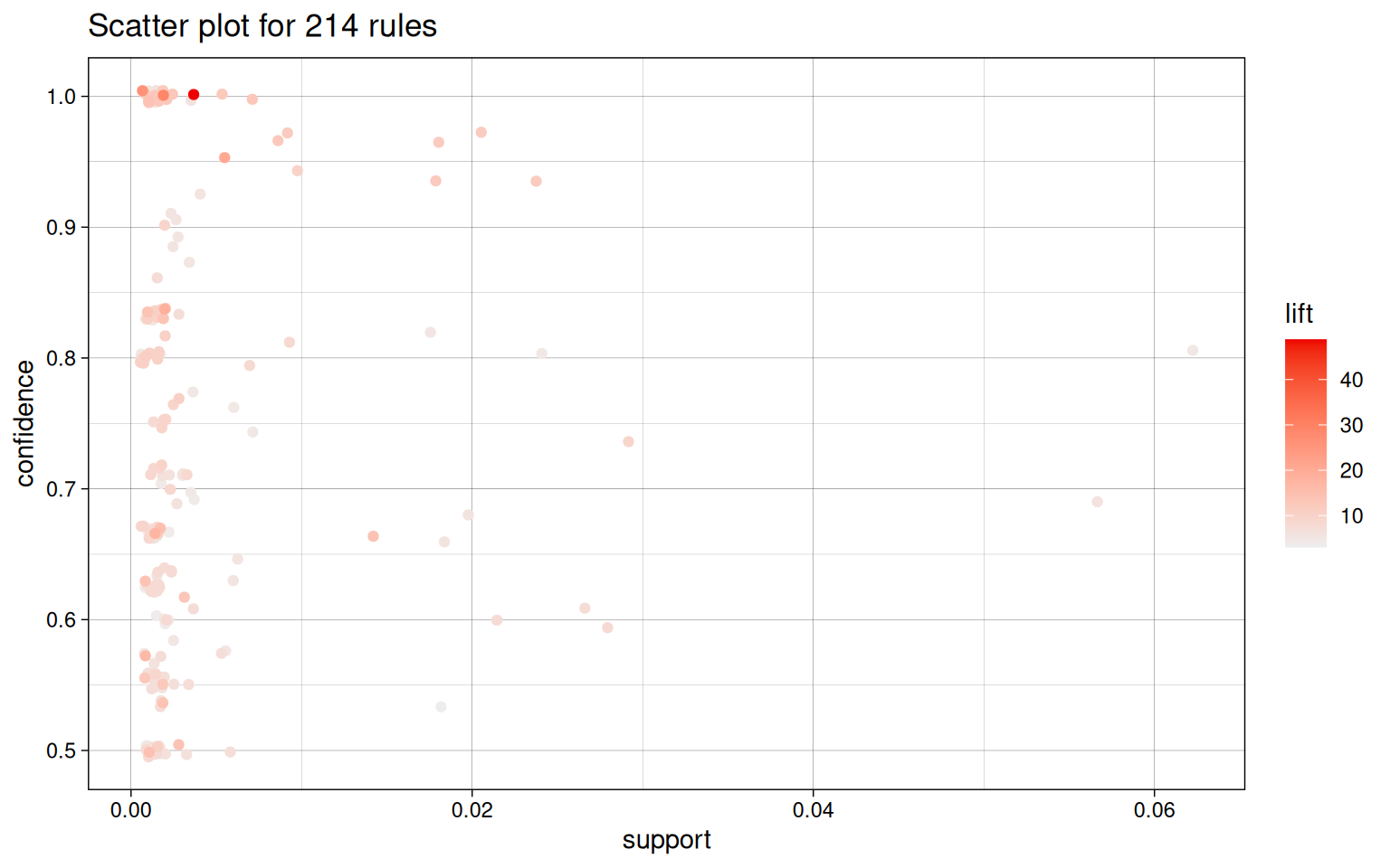
#| fig-cap: "Rule landscape: each point is one rule. Top-right corner = high support **and** high confidence (the most actionable rules)."
library(arulesViz)
plot(rules, method = "scatterplot",
     measure = c("support", "confidence"), shading = "lift",
     engine = "ggplot2")
```
## Python — `mlxtend`
The same analysis with the standard Python stack:
```{python}
#| label: apriori-python
import pandas as pd
# Pandas display: render full DataFrame width in chapter outputs.
pd.options.display.max_columns = None
pd.options.display.width = 200

from mlxtend.preprocessing import TransactionEncoder
from mlxtend.frequent_patterns import apriori, association_rules

from pathlib import Path
_data_path = "data/raw/transactions.csv" if Path("data/raw/transactions.csv").exists() else "data/synthetic/transactions.csv"
df = pd.read_csv(_data_path, sep=";")
# Drop rows whose article_name didn't survive the family-mapping (NaN or empty
# string). Mixing NaN floats with string items would crash apriori's internal
# sort with TypeError on real data.
df = df[df["article_name"].notna() & (df["article_name"].astype(str).str.strip() != "")].copy()
df["article_name"] = df["article_name"].astype(str).str.strip()
baskets = df.groupby("transaction_id")["article_name"].apply(lambda s: list(set(s))).tolist()

te = TransactionEncoder()
basket_matrix = pd.DataFrame(te.fit_transform(baskets), columns=te.columns_)

freq_items = apriori(basket_matrix, min_support=0.001, use_colnames=True)
rules = association_rules(
    freq_items, num_itemsets=len(basket_matrix),
    metric="confidence", min_threshold=0.5,
)
print(f"Total rules found: {len(rules)}")
```
### Annotating each rule for downstream views
Different stakeholders want different cuts of the same Apriori output. Cross-sell teams want pairs across product systems. Bundle-/set-merchandising wants pairs *within* the same product system. A management report wants the statistically strongest patterns regardless of category. Instead of one "actionable" filter we annotate every rule with the signals each view needs, then pick.
Signals computed:
- **Reverse confidence + symmetry score** — `min(conf(A→B), conf(B→A)) / max(...)`. Symmetric pairs (≥ 0.7) are "you can't really have one without the other" (`bett ↔ matratze`). Asymmetric pairs *can* be real cross-sell, but on real-data they often turn out to be `rare-component → main-product` (e.g. `topper → boxspringbett`) — so asymmetry alone isn't enough.
- **Within-bundle flag** — `bundle_group` of antecedent equals consequent's. Within-bundle = same product system.
- **Substring relation** — antecedent name is a substring of consequent (or vice-versa). Catches definitional component-vs-whole pairs like `auszug` and `auszugselement` that bundle-tagging alone misses on real-data variants.
- **Component-token flag** — antecedent contains a generic component/accessory token (`aufpreis`, `ablage`, `kissen`, `topper`, `aufsatz`, `element`, …). These items exist *only* as paired components of a main product — surfacing them as "cross-sell" would mislead. Curated list, real-data-derived.
- **Conviction + leverage** — additional interest metrics already provided by `mlxtend.frequent_patterns.association_rules`. Lift > 2 is the baseline for "non-trivial".
```{python}
#| label: annotate-rules
is_simple = (rules["antecedents"].apply(len) == 1) & (rules["consequents"].apply(len) == 1)
simple = (
    rules.loc[is_simple]
    .assign(
        antecedent=lambda d: d["antecedents"].apply(lambda s: next(iter(s))),
        consequent=lambda d: d["consequents"].apply(lambda s: next(iter(s))),
    )
    [["antecedent", "consequent", "support", "confidence", "lift",
      "leverage", "conviction"]]
    .reset_index(drop=True)
)

bundle_lookup = (
    df.drop_duplicates("article_name").set_index("article_name")["bundle_group"]
      .fillna("").to_dict()
)
basket_sets = df.groupby("transaction_id")["article_name"].apply(set).tolist()

def cond_prob(a, b):
    """P(a | b) — fraction of baskets containing b that also contain a."""
    n_b = sum(1 for s in basket_sets if b in s)
    if n_b == 0:
        return 0.0
    n_both = sum(1 for s in basket_sets if a in s and b in s)
    return n_both / n_b

simple["reverse_conf"] = simple.apply(
    lambda r: cond_prob(r["antecedent"], r["consequent"]), axis=1
)
simple["symmetry"] = simple.apply(
    lambda r: min(r["confidence"], r["reverse_conf"]) / max(r["confidence"], r["reverse_conf"])
        if max(r["confidence"], r["reverse_conf"]) > 0 else 0.0,
    axis=1,
)
simple["within_bundle"] = simple.apply(
    lambda r: bundle_lookup.get(r["antecedent"], "") == bundle_lookup.get(r["consequent"], "")
              and bundle_lookup.get(r["antecedent"], "") != "",
    axis=1,
)
simple["substring_pair"] = simple.apply(
    lambda r: r["antecedent"] in r["consequent"] or r["consequent"] in r["antecedent"],
    axis=1,
)

# Component / accessory tokens — curated from real-data inspection. An item
# whose name contains one of these tokens is a paired component of some main
# product, not a stand-alone item. Cross-sell rules where the antecedent is
# such a component (e.g. "topper -> boxspringbett") are definitional, not
# behavioural, and get filtered from the cross-sell view.
COMPONENT_TOKENS = {
    "aufpreis", "ablage", "aufsatz", "schublade", "schubkasten", "schubladenmodul",
    "kissen", "steckkissen", "ruckenkissen", "armlehnkissen", "armlehnenkissen",
    "nierenkissen", "klemmkissen",
    "topper", "matratze",  # mattress is a component of bed_system
    "element", "elementaufnahme", "polsterelement",
    "auszug", "auszugselement", "ansteckplatte", "tischverlangerung",
    "fusshohe", "fussteil", "sitzauszug", "querschlafer",
    "beleuchtungsset", "beleuchtung",
    "panel", "boden", "einlegeboden",
    "hakenleiste", "knopf",
    "rollcontainer",
    "sockel", "verlangerung",
    "kopfteil", "kopfstutze",
    "lattenrost",
    "ruckenelement",
    "ersatz", "ersatzteil", "zubehor", "zubehoer", "nachbestellung",
    "deko",  # "deko element" -> bed
}

def has_component_token(name):
    return bool(set(name.split()) & COMPONENT_TOKENS)

simple["component_antecedent"] = simple["antecedent"].apply(has_component_token)
simple["component_consequent"] = simple["consequent"].apply(has_component_token)
simple["component_either"] = simple["component_antecedent"] | simple["component_consequent"]

print(f"Total simple rules:          {len(simple)}")
print(f" within-bundle: {int(simple['within_bundle'].sum())}")
print(f" substring-pair: {int(simple['substring_pair'].sum())}")
print(f" component on either side: {int(simple['component_either'].sum())}")
print(f" symmetric (≥ 0.7): {int((simple['symmetry'] >= 0.7).sum())}")
print(f" lift ≥ 2 (non-trivial): {int((simple['lift'] >= 2).sum())}")
```
### View 1 — Bundle composition
*"Which items belong to the same product system?"* — useful for set-merchandising, "complete your set" UI, and inventory of complementary parts. We surface within-bundle, substring-related, *or* component-antecedent pairs, sorted by symmetry × lift so the strongest semantic pairings come out on top.
```{python}
#| label: view-bundle-composition
bundle_view = (
    simple[
        (simple["within_bundle"])
        | (simple["substring_pair"])
        | (simple["component_either"])
    ]
    .assign(score=lambda d: d["symmetry"] * d["lift"])
    .sort_values("score", ascending=False)
)
bundle_view.head(15)[["antecedent", "consequent", "support", "confidence",
                      "reverse_conf", "symmetry", "lift",
                      "within_bundle", "substring_pair", "component_either"]]\
    .round({"support": 4, "confidence": 3, "reverse_conf": 3,
            "symmetry": 2, "lift": 2})
```
### View 2 — Cross-sell
*"Which items pull in another item from a different system?"* — the deployable cross-sell-trigger list. Filter: cross-bundle (or no-bundle), no substring relation, antecedent is *not* a generic component/accessory token, asymmetric (`symmetry < 0.7`), lift ≥ 2.
```{python}
#| label: view-cross-sell
cross_sell = (
    simple[
        ~simple["within_bundle"]
        & ~simple["substring_pair"]
        & ~simple["component_either"]
        & (simple["symmetry"] < 0.7)
        & (simple["lift"] >= 2)
    ]
    .sort_values("confidence", ascending=False)
)
cross_sell.head(15)[["antecedent", "consequent", "support", "confidence",
                     "lift", "leverage", "conviction"]]\
    .round({"support": 4, "confidence": 3, "lift": 2,
            "leverage": 4, "conviction": 2})
```
These are the rules to wire into "you might also need" prompts at checkout / page-view / POS scan — antecedent demand pulls in a paired product from a different category.
### View 3 — Top insights, stratified by class
*"What are the strongest patterns in the data, period?"* — for stakeholder reports. A single global "top-N by lift" list isn't useful: definitional pairs (component → main, substring) have extreme lifts (often 100×+) and would dominate the head of the list, hiding cross-sell and within-bundle signal. We stratify instead — **top-5 per class** sorted by lift — so the reader sees the strongest representative of *each* relationship type.
```{python}
#| label: view-top-insights
def classify(r):
    if r["component_either"]:
        return "component ↔ main (definitional)"
    if r["substring_pair"]:
        return "substring (definitional)"
    if r["within_bundle"]:
        if r["symmetry"] >= 0.7:
            return "within-bundle (symmetric)"
        return "within-bundle (asymmetric)"
    if r["symmetry"] >= 0.7:
        return "symmetric (cross-bundle)"
    return "cross-sell (asymmetric)"

simple["class"] = simple.apply(classify, axis=1)
top_per_class = (
    simple.sort_values("lift", ascending=False)
          .groupby("class").head(5)
          .sort_values(["class", "lift"], ascending=[True, False])
          .reset_index(drop=True)
)
top_per_class[["class", "antecedent", "consequent", "support", "confidence",
               "lift", "conviction"]]\
    .round({"support": 4, "confidence": 3, "lift": 2, "conviction": 2})
```
```{python}
#| label: class-distribution
print("Distribution of all simple rules across classes:")
for cls, n in simple["class"].value_counts().items():
    print(f"  {cls:35s} {n}")
```
The class distribution is itself diagnostic: a healthy retail dataset has a substantial cross-sell tail (true behavioural signal), but also legitimate bundle/substring pairs (catalog plumbing). The three views above let you pick the right cut for the question at hand instead of forcing one filter to fit all three jobs.
## What each view means operationally
The methods above produce three rule lists. Each answers a different business question and feeds a different operational system. Here is what to do with each:
### View 1 — Bundle composition
**Question answered**: *"Which items are part of the same product system?"*
**What you read off it**: rules where antecedent + consequent are functional companions in one decision — bed + mattress + frame, sofa + matching cushion + element pieces, dining-table + chairs + extension. Lift here is large because the relationship is structural, not behavioural.
**Operational use cases**:
- **Set-bundling**: package the strongest within-system pairs as ready-made bundles ("Bett + Lattenrost + Matratze als Set"). The high-lift pairs are the obvious bundle candidates.
- **"Complete your set" prompts**: at checkout, if the basket has only the primary item from a set, surface the missing components.
- **Inventory coupling**: when stock of a primary item runs low, check the paired components — a stockout on the main product reduces demand for components, and vice-versa.
- **Catalog hygiene**: rules with extreme symmetry (≥ 0.9) are products you should consider merging into a single SKU or bundle, since customers don't really choose between them.
### View 2 — Cross-sell
**Question answered**: *"Which item from one product system pulls in an item from another?"*
**What you read off it**: rules where the antecedent and consequent live in *different* bundles, are *not* substring-related, and the antecedent is *not* a generic component token. These are real cross-sell triggers: the antecedent is a stand-alone product whose buyer also pulls a different stand-alone product.
**Operational use cases**:
- **Page-view recommendations**: when a customer views the antecedent product, surface the consequent in "you might also like" — but only the cross-sell view, not the bundle view, otherwise the suggestion looks redundant.
- **POS / checkout prompts**: cashier sees "TV-Schrank im Warenkorb → Highboard im Angebot anbieten".
- **Targeted email**: 14–30 days after antecedent purchase, send a follow-up offering the consequent at a small discount.
- **Floor placement**: place cross-sell pairs visually adjacent in the showroom (Sessel-Hocker-Kombination im selben Sichtbereich).
- **Cross-sell incentive plan**: if you compensate sales staff per cross-sell, this is the list of pairs that count — not the bundle pairs (those are baseline expectation, not extra effort).
### View 3 — Top insights (statistical strength)
**Question answered**: *"What are the strongest co-purchase patterns in the dataset, regardless of class?"*
**What you read off it**: rules sorted by lift, each annotated with its class — `component ↔ main`, `substring`, `within-bundle (sym/asym)`, `symmetric (cross-bundle)`, `cross-sell (asymmetric)`. The reader sees the strongest signal first, the class column tells them whether to act on it (cross-sell), package it (bundle), or note it as catalog structure (component / substring).
**Operational use cases**:
- **Stakeholder report / management presentation**: "Diese 20 Pairs erklären den Großteil der Co-Purchase-Struktur im Sortiment, hier sortiert nach Stärke und klassifiziert."
- **Methodology audit**: an analyst auditing the cross-sell list (View 2) can use View 3 as a sanity check — if a high-lift rule is missing from View 2, it's because the class column says it's bundle/substring/component, which is correct triage.
- **Catalog documentation**: the View 3 output is a snapshot of which products are tightly coupled in customer behaviour, useful for onboarding new merchandisers.
## What this chapter does *not* answer
Apriori on baskets only tells us *what is bought together*. It says nothing about:
- *Who* the buyers are (chapter 04 CLV, 06 Survival, 09 Uplift)
- *Which products dominate revenue or are growing* (chapter 02 BCG, 03 RFM)
- *What demand looks like next quarter* (chapter 07 Forecasting)
- *Which products are functionally substitutable when one is out of stock* (chapter 08 Embeddings)
The full operational picture — *which* products to push to *which* customers, *when*, with *which* offer — comes from joining the View 2 cross-sell rules with the customer-side analyses (CLV decile, win-back zone, hazard ratios) and the product-side rankings (BCG quadrants, RFM tier). That synthesis lives in [chapter 05 Insights](05-insights.qmd).
```{python}
#| label: fig-rules-python
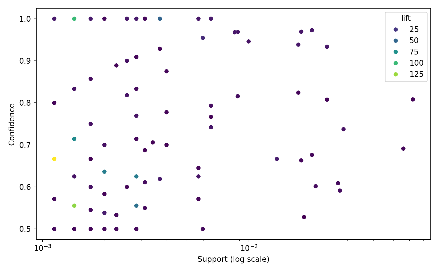
#| fig-cap: "Simple rules in support × confidence space, classified. Cross-sell rules (the actionable subset) sit visually apart from within-bundle and component-pair plumbing — the same Apriori output, shown with the triage class as colour."
import matplotlib.pyplot as plt
import seaborn as sns

# Stable class order so the legend reads top-to-bottom from "actionable" to
# "definitional plumbing".
class_order = [
    "cross-sell (asymmetric)",
    "symmetric (cross-bundle)",
    "within-bundle (asymmetric)",
    "within-bundle (symmetric)",
    "substring (definitional)",
    "component ↔ main (definitional)",
]
class_palette = {
    "cross-sell (asymmetric)":          "#27ae60",
    "symmetric (cross-bundle)":         "#3498db",
    "within-bundle (asymmetric)":       "#9b59b6",
    "within-bundle (symmetric)":        "#7f8c8d",
    "substring (definitional)":         "#f39c12",
    "component ↔ main (definitional)":  "#c0392b",
}

fig, ax = plt.subplots(figsize=(9, 5.5))
sns.scatterplot(
    data=simple, x="support", y="confidence",
    hue="class", hue_order=class_order, palette=class_palette,
    size="lift", sizes=(20, 220), alpha=0.8, ax=ax,
)
ax.set_xscale("log")
ax.set_xlabel("Support (log scale)")
ax.set_ylabel("Confidence")
ax.legend(bbox_to_anchor=(1.02, 1), loc="upper left", fontsize=8, frameon=False)
plt.tight_layout()
plt.show()
```
## R vs. Python — same answers?
Both implementations find the same total rule count and recover the same simple-rule headline patterns at identical support / confidence values — the algorithm is deterministic, not the implementation. The exact ordering of complex rules can differ when many tie on confidence (1.0), but that's a tiebreaker artifact, not a difference in what the algorithms find.
### Implementation differences worth knowing
| | `arules` (R) | `mlxtend` (Python) |
|---|---|---|
| Internal representation | sparse C-level transaction matrix | one-hot DataFrame |
| Performance on large data | very fast (10× ahead of mlxtend on 100k+ baskets) | acceptable up to ~10k baskets |
| Visualization | rich (`arulesViz`: scatter, graph, parallel coordinates, matrix) | DIY with matplotlib / networkx |
| Subsetting / pruning rules | first-class (`subset(rules, ...)`) | pandas filtering on the rules frame |
| Ecosystem fit | preferred when downstream is R / shiny | preferred when downstream is FastAPI / serving |
For exploratory work and visualization the R toolkit wins; for embedding into a Python service `mlxtend` is the easier deploy.
## Takeaway
Apriori finds raw co-purchase patterns; the work that turns those into decisions is in the postprocessing — redundancy filtering (`is.redundant`), interest measures beyond confidence (lift, conviction, leverage), and splitting the output into the views that map onto actual stakeholder questions: bundle composition, cross-sell triggers, and statistically strongest patterns. The same Apriori-run answers all three; the difference is in *which rules each view surfaces*, not in re-running the algorithm with different thresholds.