---
title: "Demand Forecasting — Monthly Revenue per Department & Category"
---
This chapter forecasts the next several months of revenue at two aggregation levels. Forecasting individual SKUs would be hopeless — too few monthly observations, too many series. We aggregate to **Category** (10 product groups, the inventory-planning level) and to **Department** (6 store-floor sections, the budget/capacity level), and demonstrate the textbook trade-off: lower aggregation gives richer drill-down, higher aggregation gives more reliable forecasts.
The honest framing of this chapter: with two years of data we sit right at the edge of what classical seasonal models can support. We get useful baselines, surface where models break down, and demonstrate the right *evaluation* discipline — which matters more in production than chasing the lowest possible MAPE on a too-small holdout.
> Tools: `statsmodels` (pure-Python, dependable). For larger datasets, `statsforecast` and `prophet` are the modern fast and ergonomic alternatives.
```{python}
#| label: setup
import warnings
warnings.filterwarnings("ignore")

import numpy as np
import pandas as pd
# Pandas display: render full DataFrame width in chapter outputs.
pd.options.display.max_columns = None
pd.options.display.width = 200

import matplotlib.pyplot as plt
import seaborn as sns
from statsmodels.tsa.statespace.sarimax import SARIMAX
from statsmodels.tsa.holtwinters import ExponentialSmoothing, SimpleExpSmoothing
import pmdarima as pm

sns.set_theme(style="whitegrid")
```
## Aggregate to monthly revenue per category
```{python}
#| label: monthly-data
from pathlib import Path
_data_path = "data/raw/transactions.csv" if Path("data/raw/transactions.csv").exists() else "data/synthetic/transactions.csv"
df = pd.read_csv(_data_path, sep=";", parse_dates=["date"])
df["month"] = df["date"].dt.to_period("M").dt.to_timestamp()

# Drop rows whose product_group / department couldn't be derived from the
# source (real data has ~5% of rows without a usable Warengruppe code).
# Keeping them would create an empty-string series in the backtest output.
df_cat  = df[df["product_group"].astype(str) != ""].copy()
df_dept = df[df["department"].astype(str)    != ""].copy()

monthly = (
    df_cat.groupby(["product_group", "month"])["gross_price"].sum()
          .unstack(fill_value=0.0)
          .stack().rename("revenue").reset_index()
          .sort_values(["product_group", "month"])
)

print(f"Categories: {monthly['product_group'].nunique()}, "
      f"Months: {monthly['month'].nunique()}, "
      f"Total rows: {len(monthly)}")

# Volume per category to pick the "well-behaved" series
totals = monthly.groupby("product_group")["revenue"].sum().sort_values(ascending=False)
print("\nTotal revenue per category:")
for cat, val in totals.items():
    print(f"  {cat}  €{val:>12,.0f}")
```
```{python}
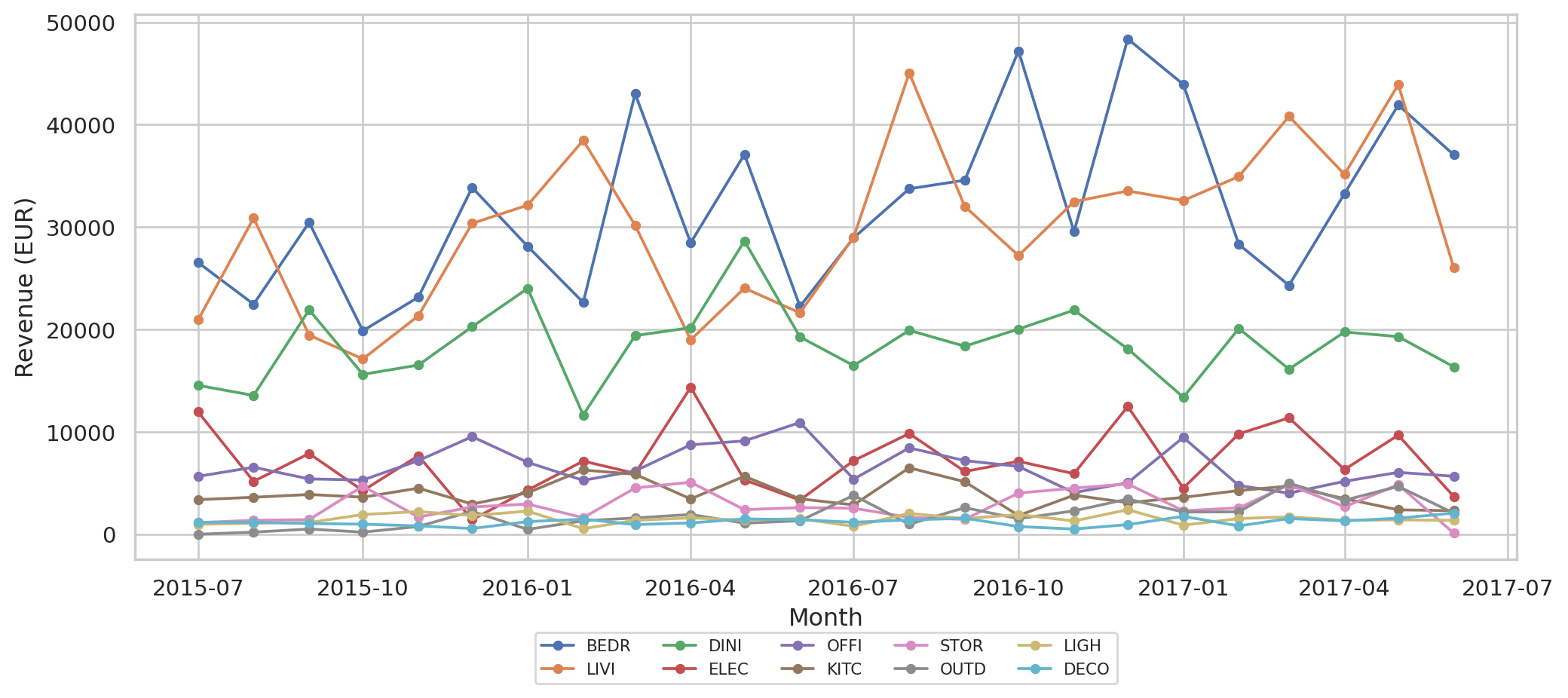
#| label: fig-series
#| fig-cap: "Monthly revenue per category. Higher-volume categories show visible seasonal-ish wobble; smaller ones are noisier. Which categories lead in revenue is data-dependent (see the per-category total printed above)."
fig, ax = plt.subplots(figsize=(11, 5))
for cat in totals.index:
    s = monthly[monthly["product_group"] == cat].set_index("month")["revenue"]
    ax.plot(s.index, s.values, marker="o", markersize=4, label=cat, lw=1.4)
ax.set_xlabel("Month")
ax.set_ylabel("Revenue (EUR)")
ax.legend(ncol=5, fontsize=8, loc="upper center", bbox_to_anchor=(0.5, -0.12))
plt.tight_layout()
plt.show()
```
The two-year window covers 1.5 seasonal cycles. That's the smallest amount on which any seasonal model has any chance — anything less and you might as well forecast with a constant.
## Models in play
| Model | What it captures | When it works |
|---|---|---|
| **Naive (last value)** | "Tomorrow looks like today" | Default benchmark; surprisingly hard to beat for short horizons |
| **Seasonal Naive** | "This month equals same month last year" | When seasonal pattern dominates noise |
| **Exponential Smoothing (ETS, no seasonality)** | Smooth trend, no seasonal component | When you have trend but too little data for seasonality |
| **Auto-ARIMA** (`pmdarima.auto_arima`) | (S)ARIMA order chosen per series via stepwise AIC search | When the order isn't known a priori — replaces a hand-picked SARIMA(1,1,1)(1,1,1,12) so each category can pick its own degrees of differencing and AR/MA orders |
We deliberately *don't* try Holt-Winters with seasonality at this point: with only ~1.5 seasonal cycles in training it almost always fails to converge. Knowing what *not* to fit is part of the discipline.
**Why Auto-ARIMA instead of a fixed order?** Hand-picking SARIMA(1,1,1)(1,1,1,12) for *every* category assumes the same dynamics across categories — clearly wrong: high-volume bedroom items behave differently from outdoor seasonals. Auto-ARIMA does a stepwise AIC search per series and lets each category pick its own (p, d, q)(P, D, Q)[m]. Standard practice in modern forecasting; saves the analyst from baking in a wrong assumption.
## Evaluation strategy
Two evaluation passes:
1. **Single 3-month holdout** (per category) — quick view of how each model would do "if we deployed today and forecast next quarter". Reported as MAE in EUR + MAPE per category × model.
2. **Rolling-origin cross-validation** — re-fit on growing training windows ending at each of the last 6 months, predict the next 3 months, average the errors. Standard practice in time series forecasting (Hyndman & Athanasopoulos, *Forecasting: Principles and Practice*) — much more robust than a single holdout. Reported as the average MAE across the rolls.
We report two metrics:
- **MAE in EUR** — absolute error in monetary terms. Stable on low-volume series.
- **MAPE** — error as percentage of actual. Easy to compare across categories *but* explodes when actuals are small (a €1k category with €500 error has MAPE 50%; same error on €100k category is 0.5%).
```{python}
#| label: backtest
HORIZON = 3

def fit_predict(train, horizon, return_intervals=False):
    """train: numpy array. Returns dict model_name -> point forecast Series.
    If return_intervals=True, also returns lower/upper 80%-CI for Auto-ARIMA."""
    out = {}
    intervals = {}

    # Naive: last train value, repeated
    out["Naive"] = pd.Series([train[-1]] * horizon, index=range(horizon))

    # Seasonal naive: same month last year (12 months back from each holdout step)
    if len(train) >= 12 + horizon:
        out["Seasonal naive"] = pd.Series(train[-12:-12 + horizon], index=range(horizon))
    else:
        out["Seasonal naive"] = pd.Series([np.nan] * horizon, index=range(horizon))

    # ETS without seasonality (just trend smoothing). Real-data series with
    # zero or near-zero months can break trend="add"; fall back to plain
    # SimpleExpSmoothing (level only) if the trended fit refuses to converge.
    # Note: statsmodels >= 0.14 removed the `disp` kwarg from .fit() — passing
    # it raises TypeError, which is why an earlier version of this code
    # silently produced all-NaN ETS forecasts.
    # ets.forecast / ses.forecast already returns a numpy array in current
    # statsmodels — no .values needed (the previous code raised AttributeError
    # silently inside the try/except, so ETS was always NaN).
    try:
        ets = ExponentialSmoothing(train, trend="add", seasonal=None,
                                   initialization_method="estimated").fit()
        out["ETS (no seasonal)"] = pd.Series(np.asarray(ets.forecast(horizon)),
                                             index=range(horizon))
    except Exception:
        try:
            ses = SimpleExpSmoothing(train, initialization_method="estimated").fit()
            out["ETS (no seasonal)"] = pd.Series(np.asarray(ses.forecast(horizon)),
                                                 index=range(horizon))
        except Exception:
            out["ETS (no seasonal)"] = pd.Series([np.nan] * horizon, index=range(horizon))

    # Auto-ARIMA — stepwise search picks (p,d,q)(P,D,Q)[12] per series
    try:
        m_season = 12 if len(train) >= 24 else 1   # seasonality only with ≥ 2 cycles
        m = pm.auto_arima(
            train, seasonal=(m_season > 1), m=m_season,
            stepwise=True, suppress_warnings=True, error_action="ignore",
            max_p=3, max_q=3, max_P=1, max_Q=1,
        )
        if return_intervals:
            yhat, conf = m.predict(horizon, return_conf_int=True, alpha=0.20)  # 80% CI
            out["Auto-ARIMA"] = pd.Series(yhat, index=range(horizon))
            intervals["Auto-ARIMA"] = (conf[:, 0], conf[:, 1])
        else:
            out["Auto-ARIMA"] = pd.Series(m.predict(horizon), index=range(horizon))
    except Exception:
        out["Auto-ARIMA"] = pd.Series([np.nan] * horizon, index=range(horizon))

    return (out, intervals) if return_intervals else out


def metrics(actual, pred):
    actual_arr = np.asarray(actual, dtype=float)
    pred_arr = np.asarray(pred, dtype=float)
    if np.isnan(pred_arr).any():
        return np.nan, np.nan
    mae = float(np.mean(np.abs(actual_arr - pred_arr)))
    # MAPE is undefined when actual=0 (real-data months with zero revenue
    # produce inf). Restrict to actual>0 entries; if none, MAPE is NaN.
    nonzero = actual_arr != 0
    if nonzero.any():
        mape = float(np.mean(np.abs((actual_arr[nonzero] - pred_arr[nonzero])
                                    / actual_arr[nonzero]))) * 100
    else:
        mape = np.nan
    return mae, mape


# --- Single 3-month holdout per category ---
rows = []
forecasts_per_cat = {}
for cat in totals.index:
    s = monthly[monthly["product_group"] == cat].set_index("month")["revenue"].asfreq("MS")
    train, test = s.iloc[:-HORIZON], s.iloc[-HORIZON:]

    preds, intervals = fit_predict(train.values, HORIZON, return_intervals=True)
    forecasts_per_cat[cat] = {"train": train, "test": test, "preds": preds,
                              "intervals": intervals}

    for model, p in preds.items():
        mae, mape = metrics(test.values, p.values)
        rows.append({"category": cat, "model": model, "MAE_EUR": mae, "MAPE_%": mape})

backtest = pd.DataFrame(rows)
```
### Rolling-origin cross-validation
Single-holdout MAE depends on which three months happened to land in the test set. Rolling-origin CV refits the model on each of the last `N_ROLLS` training-window endpoints, predicts the next `HORIZON` months, and averages — giving a much steadier error estimate per model.
```{python}
#| label: rolling-cv
N_ROLLS = 6   # last 6 different training-window endpoints

cv_rows = []
for cat in totals.index:
    s = monthly[monthly["product_group"] == cat].set_index("month")["revenue"].asfreq("MS")
    n = len(s)
    if n < 12 + HORIZON + N_ROLLS:
        continue  # not enough history for CV
    for offset in range(N_ROLLS):
        end = n - HORIZON - offset
        train_cv = s.iloc[:end]
        test_cv  = s.iloc[end:end + HORIZON]
        preds_cv = fit_predict(train_cv.values, HORIZON, return_intervals=False)
        for model, p in preds_cv.items():
            mae, _ = metrics(test_cv.values, p.values)
            cv_rows.append({"category": cat, "model": model, "roll": offset, "MAE_EUR": mae})

cv = pd.DataFrame(cv_rows)
cv_summary = cv.groupby("model")["MAE_EUR"].agg(["mean", "std", "count"]).round(0)
cv_summary.columns = ["mean MAE (EUR)", "std MAE (EUR)", "n_evaluations"]
print("Rolling-origin CV — average MAE per model across all categories × rolls:")
print(cv_summary.sort_values("mean MAE (EUR)").to_string())
```
## Per-category results
```{python}
#| label: backtest-table
pivoted_mae = backtest.pivot(index="category", columns="model", values="MAE_EUR").round(0)
pivoted_mape = backtest.pivot(index="category", columns="model", values="MAPE_%").round(1)

# Order columns sensibly
order = ["Naive", "Seasonal naive", "ETS (no seasonal)", "Auto-ARIMA"]
pivoted_mae = pivoted_mae[order]
pivoted_mape = pivoted_mape[order]

print("MAE (EUR) per category × model:")
print(pivoted_mae.to_string())
print()
print("MAPE (%) per category × model:")
print(pivoted_mape.to_string())
```
```{python}
#| label: aggregate-metrics
overall = backtest.groupby("model")[["MAE_EUR", "MAPE_%"]].mean().round(1)
overall["wins"] = backtest.loc[backtest.groupby("category")["MAE_EUR"].idxmin(), "model"]\
                          .value_counts().reindex(overall.index, fill_value=0)
overall = overall.reindex(order)
overall
```
A few patterns emerge:
- **Naive (last value)** is shockingly competitive on short horizons. With 3 months of forecast, last-month-anchored prediction often beats more sophisticated models — a classic finding in the forecasting literature.
- **Seasonal naive** wins on categories with clearer annual seasonality (garden / outdoor goods, dining items around holiday months).
- **Auto-ARIMA** sometimes overfits the limited training history and produces worse-than-naive forecasts. The stepwise AIC search picks the best order *for the training period*, which on short series is not necessarily the best order *for the future*.
- **MAPE** is misleading for the smallest categories — a 100% MAPE on STOR (low-volume storage) is a few thousand euros of error, not a forecasting catastrophe.
## Granularity matters — Department vs. Category
The above runs at *Category* level (~10 series — `product_group`). The catalog also has a *Department* level above category (6 series), which aggregates across related categories. With the same monthly window, Department-level series have **roughly the noise floor halved** — `Living` for example combines `LIVI + DECO + LIGH + ELEC`, so randomness in any one category averages out.
```{python}
#| label: department-backtest
monthly_dept = (
    df_dept.groupby(["department", "month"])["gross_price"].sum()
           .unstack(fill_value=0).stack().rename("revenue").reset_index()
           .sort_values(["department", "month"])
)

dept_rows = []
for dept in sorted(monthly_dept["department"].unique()):
    s = monthly_dept[monthly_dept["department"] == dept].set_index("month")["revenue"].asfreq("MS")
    train, test = s.iloc[:-HORIZON], s.iloc[-HORIZON:]
    preds = fit_predict(train.values, HORIZON)
    for model, p in preds.items():
        mae, mape = metrics(test.values, p.values)
        dept_rows.append({"level": "Department", "series": dept, "model": model,
                          "MAE_EUR": mae, "MAPE_%": mape})

# Re-tag the original category backtest for comparison
cat_rows = backtest.copy()
cat_rows["level"] = "Category"
cat_rows = cat_rows.rename(columns={"category": "series"})[["level", "series", "model", "MAE_EUR", "MAPE_%"]]

combined = pd.concat([pd.DataFrame(dept_rows), cat_rows], ignore_index=True)
summary = combined.groupby(["level", "model"])[["MAE_EUR", "MAPE_%"]].mean().round(1)
summary
```
```{python}
#| label: fig-level-compare
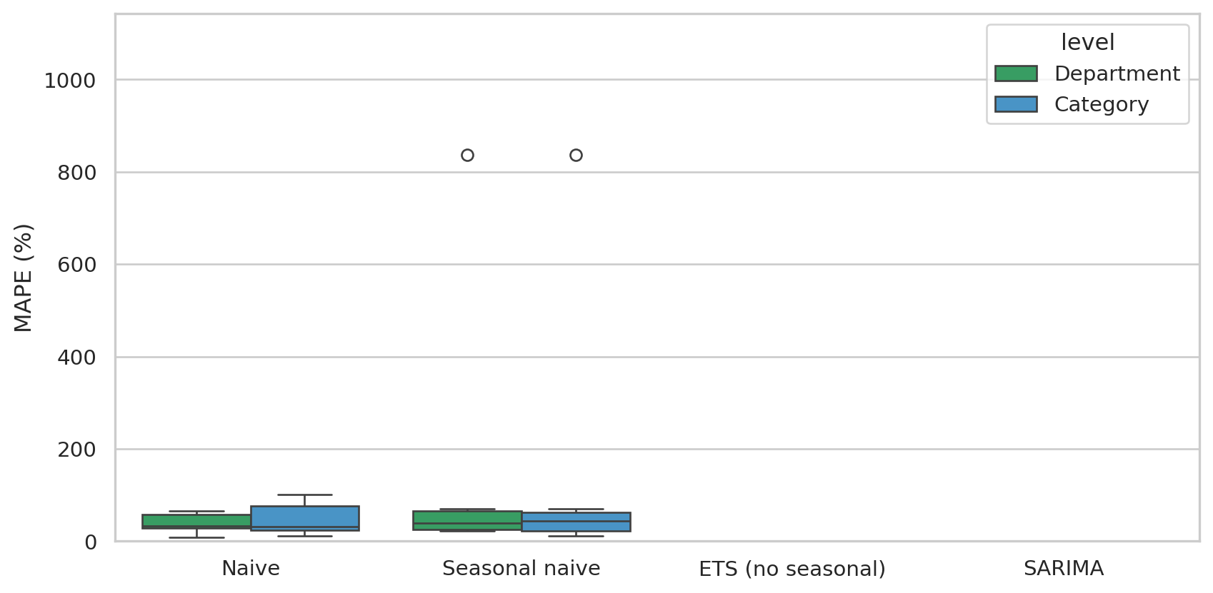
#| fig-cap: "MAPE distribution per model at Category vs. Department level. Department-level forecasts are tighter — the same models work better when the series has more signal-to-noise."
fig, ax = plt.subplots(figsize=(9, 4.5))
sns.boxplot(data=combined, x="model", y="MAPE_%", hue="level", ax=ax,
            order=order, palette={"Category": "#3498db", "Department": "#27ae60"})
ax.set_ylabel("MAPE (%)")
ax.set_xlabel("")
ax.set_ylim(0, max(60, combined["MAPE_%"].quantile(0.95)))
plt.tight_layout()
plt.show()
```
This is the textbook trade-off in hierarchical forecasting: **higher granularity = more interpretable, lower signal**; **higher aggregation = less interpretable, more reliable**. In production you'd usually:
1. Forecast at **Department level** for budget / capacity / supplier negotiations (the "is the business growing?" question).
2. Forecast at **Category level** for inventory and promotional planning (the "how many garden tables in March?" question).
3. **Reconcile** so the per-category forecasts sum to the department forecast — there are libraries like Nixtla's `hierarchicalforecast` for exactly this.
We don't reconcile here (the ~24-month window is too thin to demonstrate it well), but the takeaway sticks: the right level of granularity is *the one the decision needs*, not always the finest available.
## Forecast vs. actual — three representative categories
```{python}
#| label: fig-forecast-compare
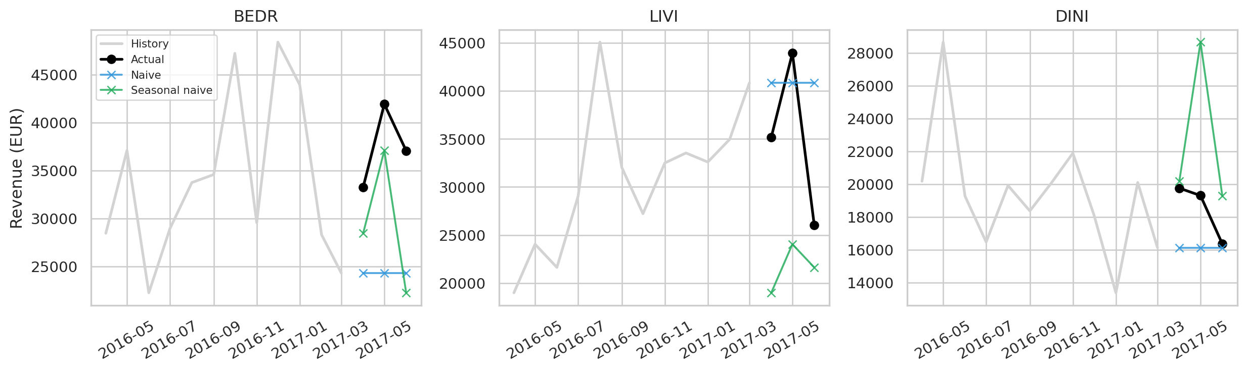
#| fig-cap: "Forecast vs. actual on the last three months for the three highest-volume categories. Black points = the actual; coloured lines = each model's point forecast. The red shaded band is the Auto-ARIMA 80 % prediction interval — reading inventory decisions off point forecasts alone hides that the truth could land anywhere inside this band."
top_cats = totals.index[:3].tolist()
fig, axes = plt.subplots(1, 3, figsize=(13, 4), sharey=False)

for ax, cat in zip(axes, top_cats):
    ctx = forecasts_per_cat[cat]
    train, test = ctx["train"], ctx["test"]
    intervals = ctx.get("intervals", {})

    # Plot trailing 12 months of train + actual
    train_tail = train.iloc[-12:]
    ax.plot(train_tail.index, train_tail.values, color="lightgrey", lw=2, label="History")
    ax.plot(test.index, test.values, color="black", marker="o", lw=2, label="Actual")

    # Auto-ARIMA prediction interval shaded
    if "Auto-ARIMA" in intervals:
        lo, hi = intervals["Auto-ARIMA"]
        ax.fill_between(test.index, lo, hi, color="#c0392b", alpha=0.15,
                        label="Auto-ARIMA 80% CI")

    colors = {"Naive": "#3498db", "Seasonal naive": "#27ae60",
              "ETS (no seasonal)": "#f39c12", "Auto-ARIMA": "#c0392b"}
    for model, p in ctx["preds"].items():
        if np.isnan(p.values).any():
            continue
        ax.plot(test.index, p.values, marker="x", lw=1.4,
                color=colors.get(model, "grey"), label=model, alpha=0.85)

    ax.set_title(cat)
    ax.tick_params(axis="x", rotation=30)
    if cat == top_cats[0]:
        ax.legend(fontsize=7, loc="upper left")
        ax.set_ylabel("Revenue (EUR)")

plt.tight_layout()
plt.show()
```
## Why "boring baselines beat fancy models" here
The takeaway from forecasting research over the last 40 years (M-competitions, Makridakis et al.) is consistent: on short horizons with little history, simple models are *frequently better than ML/deep learning*. Three reasons play out in this dataset:
1. **Bias-variance** — sophisticated models have many parameters. With 21 months of training, parameter estimates are noisy. Naive has zero parameters; it can't overfit.
2. **No exogenous regressors** — we forecast on revenue alone. ARIMA-class models and ETS have nothing to cling to except the autocorrelation in the series, which is weak with monthly retail data.
3. **Heterogeneity** — 10 categories, each with its own dynamic. A single model class often doesn't fit all of them; per-category model selection (or hierarchical pooling) helps a lot but needs more data than we have.
For *this* dataset, the right operational approach would be:
- **Use seasonal naive as the production baseline** — it captures the dominant signal (annual cyclicality) with zero training time.
- **Reserve Auto-ARIMA / ETS for categories where they clearly outperform** — measure per category × roll, switch only on persistent improvement (rolling-origin CV captures this).
- **Don't trust point forecasts blindly** — plan inventory with prediction intervals (the Auto-ARIMA panels in *Forecast vs. actual* below show 80 % CIs as shaded bands) to express the true uncertainty.
## Limitations
- **~24 months is genuinely too few** for confident seasonal modeling. In production, you'd want 3–5 years.
- **Synthetic data has no embedded seasonality**. Our generator produces uniform-in-time transactions modulo trend; real retail has strong holiday peaks (Christmas, Easter, summer for outdoor) that would make seasonal models far more useful than they appear here.
- **Cross-category dependencies aren't modeled**. Hierarchical / multivariate models (e.g. VAR, hierarchical reconciliation in `hierarchicalforecast`) would exploit shared structure across categories.
- **Single 80 % CI per Auto-ARIMA**. The plot shows the Auto-ARIMA-derived interval; the naive / seasonal-naive / ETS panels would also benefit from interval reporting (e.g. via the residual-bootstrap approach), which we don't show here.
## How this chapter fits the rest
| Chapter | Time direction | Output |
|---|---|---|
| 04 — CLV (BG/NBD) | Forward, per customer | Expected per-customer purchases & revenue |
| 06 — Survival | Forward, per customer | When does the return probability decay? |
| 07 — Forecasting (this) | Forward, per category | Aggregate revenue trajectory |
CLV and Survival are *individual*; Forecasting is *aggregate*. A retailer needs both: CLV/Survival to decide whom to target with personalized offers, Forecasting to decide *how much stock to order* and *what budget to plan*.