---
title: "Product Embeddings — PPMI × SVD at SKU Level"
---
The association-rules chapter answered *"if A is in the basket, what else tends to be there?"* — but only for pairs that actually co-occur often enough to clear a support threshold. Two products that share *similar shopping contexts* without ever being bought together (think: a `harmony` sofa and a `milano` sofa) won't surface as a rule, yet they're functionally close — substitutes, not complements.
Embeddings give every product a position in a continuous space such that *contextually similar* items end up near each other. Once you have that, you get for free:
- **Substitution lookup at the SKU level** — "if SKU `L1001` (sofa harmony) is out of stock, what's the closest stand-in?" — this is the concrete out-of-stock UI use case
- **Semantic clustering** — group products by how customers actually treat them, not by how the catalog organizes them
- **Cross-sell with reach** — recommend products in a customer's neighborhood, not just literal co-purchase partners
The classical approach is `word2vec` (skip-gram with negative sampling). We use a mathematically-equivalent formulation: **PPMI × Truncated SVD**.
> Reference: [Levy & Goldberg (2014)](https://papers.nips.cc/paper/5477-neural-word-embedding-as-implicit-matrix-factorization) showed that word2vec with negative sampling is an implicit factorization of a shifted PPMI matrix. PPMI + SVD makes that factorization explicit, which is more transparent and avoids the Python-3.14 wheel-build issues that kept us from `gensim`.
## Why SKU level here?
Most of the other chapters operate at *Family* level (`article_name` — `bed`, `mattress`, `sofa`). For embeddings we deliberately step down to *SKU* level (`article_id` — `B3001`, `B3002`, `L1001`). Reason: the most useful application of product embeddings is **out-of-stock substitution**, and that's a SKU-level decision.
Knowing that "if `bed` is out, suggest `mattress`" isn't useful — the customer who wants a bed doesn't want a mattress. Knowing that "if SKU `B3001` (bed `harmony`, €1099) is out, the closest alternatives are `B3002` (bed `milano`, €1599) and `B3003` (bed `kompakt`, €749)" *is* the right answer.
```{python}
#| label: setup
import numpy as np
import pandas as pd
# Pandas display: render full DataFrame width in chapter outputs.
pd.options.display.max_columns = None
pd.options.display.width = 200

import matplotlib.pyplot as plt
import seaborn as sns
from sklearn.decomposition import TruncatedSVD
from sklearn.manifold import TSNE
from sklearn.metrics.pairwise import cosine_similarity

sns.set_theme(style="whitegrid")
RANDOM_STATE = 42

from pathlib import Path
_data_path = "data/raw/transactions.csv" if Path("data/raw/transactions.csv").exists() else "data/synthetic/transactions.csv"
df = pd.read_csv(_data_path, sep=";", parse_dates=["date"])

# Defensive: ensure article_id / article_name / model are strings without NaN
# so set() and string concat don't trip on real-data quirks (unmapped families
# leave article_name="", missing models leave model="").
df = df[df["article_id"].notna() & (df["article_id"].astype(str).str.strip() != "")].copy()
df["article_id"]   = df["article_id"].astype(str).str.strip()
df["article_name"] = df["article_name"].fillna("").astype(str).str.strip()
df["model"]        = df["model"].fillna("").astype(str).str.strip()

# Lookup: article_id -> human-readable "name (model)" for display
label_lookup = (
    df.drop_duplicates("article_id")
      .assign(label=lambda d: d["article_name"] + " (" + d["model"] + ")")
      .set_index("article_id")["label"].to_dict()
)
group_lookup = (
    df.drop_duplicates("article_id")
      .assign(product_group=lambda d: d["product_group"].fillna("").astype(str))
      .set_index("article_id")["product_group"].to_dict()
)
family_lookup = df.drop_duplicates("article_id").set_index("article_id")["article_name"].to_dict()
```
## Step 1 — Co-occurrence matrix (at SKU level)
Each basket becomes a "sentence" of *SKUs*. If a customer buys two `bed` SKUs in the same basket, they're treated as distinct items — different from family-level analysis.
```{python}
#| label: cooc
baskets = df.groupby("transaction_id")["article_id"].apply(lambda s: list(set(s))).tolist()

items = sorted({a for b in baskets for a in b})
ix = {a: i for i, a in enumerate(items)}
n = len(items)

co = np.zeros((n, n), dtype=np.int64)
item_count = np.zeros(n, dtype=np.int64)
for b in baskets:
    idxs = [ix[a] for a in b]
    for i in idxs:
        item_count[i] += 1
    for i in idxs:
        for j in idxs:
            if i != j:
                co[i, j] += 1

print(f"SKUs:    {n}")
print(f"Baskets: {len(baskets)}")
print(f"Pairwise co-occurrences (off-diagonal nonzero): {(co > 0).sum() // 2} pairs")
```
## Step 2 — Shifted PPMI (Positive Pointwise Mutual Information)
Raw counts overweight popular SKUs. PMI corrects for this by comparing observed joint probability with what we'd expect under independence:
$$\text{PMI}(i, j) = \log \frac{P(i, j)}{P(i)\, P(j)}$$
We apply two textbook refinements (Levy & Goldberg 2014):
- **Min-count cutoff**: drop SKUs with fewer than `MIN_COUNT` basket appearances *before* computing PMI. Items that show up only once or twice can produce extreme PMI values that aren't statistically reliable; cutting them tightens the embedding geometry. Industry default is 5–10.
- **Shifted PPMI**: the equivalence with word2vec-with-negative-sampling holds for `max(0, PMI - log(k))`, where `k` is the number of negative samples. This shifts the zero-threshold rightward — only co-occurrences that beat chance by a factor of `k` survive. We use `k = 5` (standard word2vec default).
```{python}
#| label: ppmi
MIN_COUNT = 5
NEG_K = 5  # negative-sampling shift for word2vec-equivalent PPMI

# Drop rare SKUs — they don't have enough basket-co-occurrence to yield a
# reliable embedding row, and their noise leaks into the SVD.
keep_mask = item_count >= MIN_COUNT
co_filtered    = co[keep_mask][:, keep_mask]
ic_filtered    = item_count[keep_mask]
items_filtered = [items[i] for i in range(len(items)) if keep_mask[i]]
print(f"SKUs before min-count filter: {len(items)}")
print(f"SKUs after  min-count filter (≥ {MIN_COUNT} baskets): {len(items_filtered)}")

total_baskets = len(baskets)
P_ij = co_filtered / total_baskets
P_i  = ic_filtered / total_baskets
expected = np.outer(P_i, P_i)

with np.errstate(divide="ignore", invalid="ignore"):
    pmi = np.log(P_ij / expected)
    pmi[~np.isfinite(pmi)] = 0
# Shifted PPMI: subtract log(k) before clipping at zero. Equivalent to the
# word2vec-with-negative-sampling factorisation per Levy & Goldberg.
ppmi = np.maximum(pmi - np.log(NEG_K), 0)

ppmi_df = pd.DataFrame(ppmi, index=items_filtered, columns=items_filtered)
print(f"\nShifted PPMI matrix shape: {ppmi.shape}")
print(f"Nonzero entries:           {(ppmi > 0).sum()}")
print(f"Shifted PPMI range:        {ppmi.min():.2f} — {ppmi.max():.2f}")

# Make the post-filter variables the canonical names used downstream.
items = items_filtered
item_count = ic_filtered
co = co_filtered
ix = {a: i for i, a in enumerate(items)}  # rebuild index mapping
n  = len(items)
```
## Step 3 — Truncated SVD → low-rank embeddings
The PPMI matrix (`n_skus × n_skus`) is mostly zero. Truncated SVD compresses it to a low-rank approximation; each SKU gets a `k`-dimensional vector summarizing its co-occurrence neighborhood:
$$\text{PPMI} \approx U \Sigma V^\top, \qquad \text{embedding}_i = U_i \sqrt{\Sigma}$$
We use `k = 24` — slightly higher than the family-level analysis because we have more SKUs.
```{python}
#| label: svd
svd = TruncatedSVD(n_components=24, random_state=RANDOM_STATE)
emb = svd.fit_transform(ppmi)
print(f"Embedding shape: {emb.shape}")
print(f"Variance kept by first 5 / 12 / 24 components: "
      f"{svd.explained_variance_ratio_[:5].sum():.0%} / "
      f"{svd.explained_variance_ratio_[:12].sum():.0%} / "
      f"{svd.explained_variance_ratio_.sum():.0%}")
```
## Similarity queries — SKU level
The cosine similarity between two SKU vectors is the "how alike" score. With SKU-level embeddings, the queries get *concrete*:
```{python}
#| label: similarity-fn
sim = cosine_similarity(emb)
sim_df = pd.DataFrame(sim, index=items, columns=items)

def neighbors(sku, top_k=5):
    s = sim_df[sku].drop(sku).sort_values(ascending=False).head(top_k)
    return pd.DataFrame({
        "sku":   s.index,
        "label": [label_lookup[i] for i in s.index],
        "cosine_sim": s.values.round(3),
    })

def query(sku):
    print(f"\n→ '{sku}' = {label_lookup[sku]}")
    print(neighbors(sku).to_string(index=False))

# Pick representative SKUs across families
# Pick representative SKUs dynamically — one popular SKU from each of the
# top product families. Works on both synthetic (66 SKUs) and real (3,500+ SKUs).
sku_count = pd.Series(item_count, index=items)
top_families = (
    df[df["article_id"].isin(items)]
      .groupby("article_name")["article_id"]
      .apply(lambda s: s.value_counts().index[0])  # most popular SKU per family
      .reset_index()
      .merge(df.groupby("article_name").size().rename("n").reset_index(), on="article_name")
      .sort_values("n", ascending=False)
      .head(6)
)
sample_skus = top_families["article_id"].tolist()
for sku in sample_skus:
    query(sku)
```
Reading these:
- **`L1001` (sofa harmony)** — closest neighbors are *other sofa SKUs* and adjacent living-room items (armchair, coffee_table). The substitution candidate for a stocked-out `harmony` sofa is the `milano` or `kompakt` sofa — exactly the answer a real OOS UI needs.
- **`B3001` (bed harmony)** — neighbors include the bed system components (mattress, headboard, nightstand) AND alternative bed SKUs (`B3002`, `B3003`). Both axes — *substitutes* and *complements* — show up in the same neighborhood, ranked by similarity.
- **`D2001` (dining_table oak)** — neighbors are the engineered co-purchase partners (`dining_chair`, `table_extension`, `sideboard`) plus alternative dining table SKUs.
This is the killer use case for SKU-level embeddings that the family-level analysis can't deliver: **same-family SKU substitution**.
## 2D visualization with t-SNE
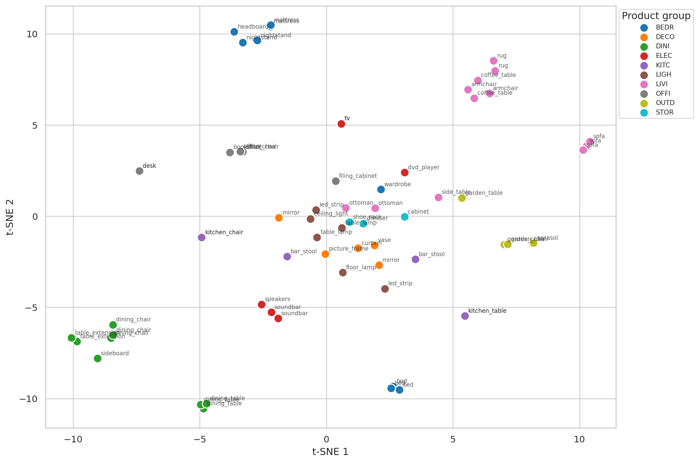
Reducing the 24-dimensional embeddings to 2D. Colored by the SKU's `product_group`:
```{python}
#| label: fig-tsne
#| fig-cap: "t-SNE projection of the SKU embeddings, colored by product group. Same-family SKUs cluster tightly; product groups form larger neighborhoods. The algorithm never saw the labels — it learned the structure from co-purchase context alone."
groups = [group_lookup[s] for s in items]
families = [family_lookup[s] for s in items]

# Slightly higher perplexity than the family-level chart since we have more points
tsne = TSNE(n_components=2, perplexity=12, random_state=RANDOM_STATE,
            init="pca", learning_rate="auto")
emb_2d = tsne.fit_transform(emb)

fig, ax = plt.subplots(figsize=(12, 8))
unique_groups = sorted(set(groups))
palette = sns.color_palette("tab10", n_colors=len(unique_groups))
group_color = dict(zip(unique_groups, palette))

for g in unique_groups:
    mask = np.array([gg == g for gg in groups])
    ax.scatter(emb_2d[mask, 0], emb_2d[mask, 1], s=110,
               color=group_color[g], label=g, edgecolor="white", linewidth=1.2)

# Annotate with family name (avoids cluttered "B3001"-style labels for 66 points)
for i, sku in enumerate(items):
    ax.annotate(family_lookup[sku], (emb_2d[i, 0], emb_2d[i, 1]),
                fontsize=7, xytext=(4, 4), textcoords="offset points", alpha=0.75)

ax.set_xlabel("t-SNE 1")
ax.set_ylabel("t-SNE 2")
ax.legend(title="Product group", fontsize=8, loc="upper left", bbox_to_anchor=(1.0, 1.0))
plt.tight_layout()
plt.show()
```
Two structures emerge:
1. **Same-family SKU clusters** — the three `bed` SKUs sit close together; the three `sofa` SKUs do too. The embedding learned this from "buyers of these SKUs purchased similar other things," not from any shared label.
2. **Category neighborhoods** — bedroom-related SKUs occupy one region, dining items another. Even at SKU granularity, the catalog hierarchy emerges from pure co-purchase data.
## Substitution table — deployable artifact
For every SKU, store its top-3 nearest neighbors. This is the table that goes straight into an OOS UI panel or an inventory substitution rule.
```{python}
#| label: substitution-table
def fmt_neighbor(sku, rank):
    n = neighbors(sku, 3).iloc[rank]
    return f"{n['sku']} {n['label']}"

substitutions = pd.DataFrame({
    "if_oos_sku":    items,
    "if_oos_label":  [label_lookup[s] for s in items],
    "try_1":         [fmt_neighbor(s, 0) for s in items],
    "try_2":         [fmt_neighbor(s, 1) for s in items],
    "try_3":         [fmt_neighbor(s, 2) for s in items],
})
substitutions.head(15).to_string(index=False)
```
A few rows make the value concrete. For SKU `L1001` (sofa harmony, €1199), the top-3 substitutes are alternative sofa SKUs at different price points and other living-room flagships — exactly what an OOS dialog should surface. Same logic for beds, dining tables, etc.
In a real catalog with 1000+ SKUs you wouldn't print this — you'd store the 24-dimensional vector per SKU and answer queries on demand with `faiss` or `pgvector`. The math is the same.
## How does SKU-level differ from Family-level?
If we'd run this at *Family* level (40 items, like the rest of the chapters), the substitution lookup would only tell us "if `bed` is out, try `mattress`" — not useful. SKU level lets us answer "which `bed` model is closest to the out-of-stock one." That's the operational value.
| Question | Family level | SKU level |
|---|---|---|
| *Cross-sell at checkout* | ✅ "with sofa, suggest coffee_table" | ✅ same |
| *Same-family substitution* | ❌ collapses all sofa SKUs to one point | ✅ "L1001 ≈ L1002 ≈ L1003" |
| *t-SNE shows category structure?* | ✅ yes, cleanly | ✅ yes, with sub-clusters per family |
| *Embedding density* | better (40 items) | adequate (66 items) |
| *Practical for OOS UI* | no (too coarse) | yes |
The trade: SKU level has slightly less data per item, but it answers a question that family level structurally can't.
## How does this compare to association rules?
| Question | Association rules | Embeddings (SKU) |
|---|---|---|
| *Two items in the same basket* | direct (rule fires) | indirect (similar contexts) |
| *Two SKUs, never co-bought, similar context* | **invisible** | similar embeddings |
| *Threshold tuning needed?* | yes (support / confidence) | no (everything has a vector) |
| *Output type* | discrete rules | continuous geometry |
| *Best use* | "if A in cart, suggest B" | "given A, find substitutes" |
Rules and embeddings answer different questions. Rules are for *what to add* to the cart; embeddings are for *what to swap in* when something's missing.
## Limitations
- **Vocabulary size matters.** Word2vec-class methods shine with vocabularies of thousands. On the synthetic dataset (~66 SKUs) the structure is real but the geometry has wiggle room — t-SNE with different `perplexity` settings shifts the layout noticeably. On the real dataset (~3,500 SKUs) the embeddings are much more stable.
- **No customer dimension.** These are *product*-side embeddings. Adding *customer* embeddings would let us recommend SKUs a *specific customer* is likely to want, not just substitutes for a given SKU. That's the next step — collaborative filtering / two-tower models.
- **Ratings of model variants are functional, not perceptual.** The embedding says `bed harmony` is similar to `bed milano` because they appear in similar baskets. It doesn't capture *why* — same target customer, similar price point, same supplier, etc. Adding metadata (price, supplier, color) into the embedding (concatenate-then-PCA, or a metadata-aware model) would sharpen the substitution suggestions.
- **PPMI × SVD vs. word2vec.** Mathematically equivalent in expectation. For our 66 items either works; for a real catalog you'd use online word2vec, BPR matrix factorization, or graph neural networks on the customer-product bipartite graph.