---
title: "Customer Lifetime Value — BG/NBD + Gamma-Gamma"
---
The clustering chapters answered *which products are healthy* and *which customer segments exist*. This chapter answers a sharper question: **how much is each individual customer worth, and how confident are we?**
We use two probabilistic models that are the standard for *non-contractual* retail (i.e. customers can leave at any time without notice):
- **BG/NBD** — predicts *how many* future purchases each customer will make, plus their probability of still being "alive" (not silently churned). The model assumes customer transactions while alive follow a Poisson process with a Gamma-distributed rate, and lifetime is exponentially distributed with a Beta-distributed dropout probability.
- **Gamma-Gamma** — predicts the *average value* of each future purchase, independent of how many they make. Assumes monetary values per transaction are Gamma-distributed and uncorrelated with frequency.
Combining the two gives expected revenue per customer over a chosen horizon — the *Customer Lifetime Value*.
> Reference: [Fader, Hardie & Lee (2005)](https://www.brucehardie.com/papers/bgnbd_2004-04-20.pdf) for BG/NBD; [Fader & Hardie (2013)](https://www.brucehardie.com/notes/025/) for Gamma-Gamma. Implementation via the [`lifetimes`](https://lifetimes.readthedocs.io/) Python package.
```{python}
#| label: setup
import numpy as np
import pandas as pd
# Pandas display: render full DataFrame width in chapter outputs.
pd.options.display.max_columns = None
pd.options.display.width = 200

import matplotlib.pyplot as plt
import seaborn as sns
from lifetimes import BetaGeoFitter, GammaGammaFitter
from lifetimes.utils import (
    summary_data_from_transaction_data,
    calibration_and_holdout_data,
)

sns.set_theme(style="whitegrid")
```
## From line items to (frequency, recency, T)
BG/NBD doesn't care about baskets — it works with three numbers per customer:
- **frequency** — number of *repeat* transactions (excluding the first; one-time buyers have frequency 0)
- **recency** — days between first and last transaction (0 for one-time buyers)
- **T** — days between first transaction and the observation end
Per-transaction monetary value comes from the basket gross price.
```{python}
#| label: data-prep
from pathlib import Path
_data_path = "data/raw/transactions.csv" if Path("data/raw/transactions.csv").exists() else "data/synthetic/transactions.csv"
df = pd.read_csv(_data_path, sep=";", parse_dates=["date"])

# Aggregate line items to one row per (customer, transaction)
tx = (
    df.groupby(["customer_id", "transaction_id", "date"], as_index=False)
      ["gross_price"].sum()
)
print(f"{len(tx)} transactions across {tx['customer_id'].nunique()} customers")

OBS_END = tx["date"].max()
summary = summary_data_from_transaction_data(
    tx,
    customer_id_col="customer_id",
    datetime_col="date",
    monetary_value_col="gross_price",
    observation_period_end=OBS_END,
    freq="D",
)
summary.head()
```
```{python}
#| label: summary-stats
n_total = len(summary)
n_returning = (summary["frequency"] >= 1).sum()
print(f"Customers in summary:      {n_total}")
print(f"  one-time buyers:         {n_total - n_returning}  ({(n_total - n_returning)/n_total:.1%})")
print(f"  returning (freq >= 1):   {n_returning}  ({n_returning/n_total:.1%})")
print()
print("Distribution of frequencies (repeat purchases per customer):")
print(summary["frequency"].value_counts().sort_index().head(10))
```
A heavy-tailed split between one-time and returning customers — typically 60–80 % one-time in retail data — is exactly the regime BG/NBD was designed for. The exact ratio in the printed summary above depends on which dataset is loaded.
## Fit BG/NBD
```{python}
#| label: fit-bgnbd
bgf = BetaGeoFitter(penalizer_coef=0.001)
bgf.fit(summary["frequency"], summary["recency"], summary["T"])
bgf.summary.round(3)
```
The four parameters describe the *population*:
- **r, α** — shape and scale of the Gamma distribution of transaction rates across customers (heterogeneity in *purchasing* behavior)
- **a, b** — Beta distribution governing the per-transaction dropout probability (heterogeneity in *lifetime* behavior)
The values say roughly: most customers have low transaction rates, but some are much more active than others; once a customer is inactive for a stretch comparable to their typical inter-purchase time, dropout becomes likely.
### Holdout validation
A model that fits the past well isn't useful unless it predicts the future. We split the timeline: fit on the first 18 months, evaluate predictions over the last 6 months.
```{python}
#| label: holdout
CAL_END = OBS_END - pd.Timedelta(days=180)

cal_holdout = calibration_and_holdout_data(
    tx,
    customer_id_col="customer_id",
    datetime_col="date",
    monetary_value_col="gross_price",
    calibration_period_end=CAL_END,
    observation_period_end=OBS_END,
    freq="D",
)

bgf_cal = BetaGeoFitter(penalizer_coef=0.001)
bgf_cal.fit(
    cal_holdout["frequency_cal"],
    cal_holdout["recency_cal"],
    cal_holdout["T_cal"],
)

cal_holdout["predicted_holdout"] = (
    bgf_cal.conditional_expected_number_of_purchases_up_to_time(
        180,
        cal_holdout["frequency_cal"],
        cal_holdout["recency_cal"],
        cal_holdout["T_cal"],
    )
)
print(f"Customers in calibration sample: {len(cal_holdout)}")
print(f"Holdout window:                  {180} days")
print(
    f"Total purchases in holdout:      {int(cal_holdout['frequency_holdout'].sum())} actual, "
    f"{cal_holdout['predicted_holdout'].sum():.0f} predicted"
)
```
```{python}
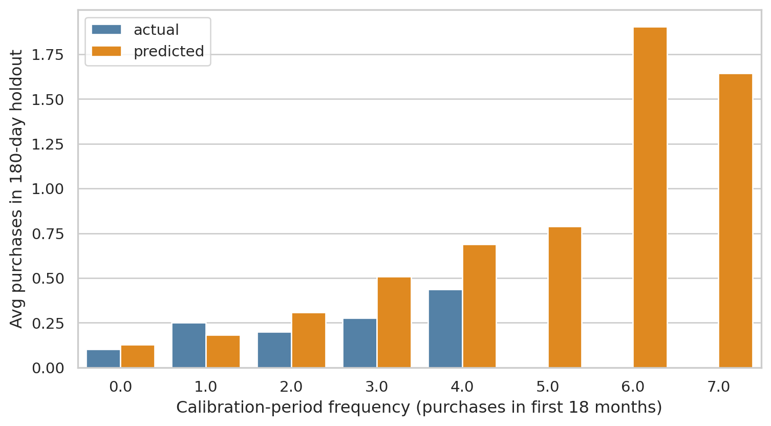
#| label: fig-holdout
#| fig-cap: "Holdout calibration. Each point is a calibration-frequency bin (number of purchases the customer made in the first 18 months). The model's predicted holdout purchases (orange) tracks the actual (blue) closely — the BG/NBD assumptions fit this dataset well."
agg = (
    cal_holdout.groupby("frequency_cal")
    .agg(
        n=("frequency_holdout", "size"),
        actual=("frequency_holdout", "mean"),
        predicted=("predicted_holdout", "mean"),
    )
    .reset_index()
)

fig, ax = plt.subplots(figsize=(8, 4.5))
agg_long = agg.melt(
    id_vars=["frequency_cal", "n"],
    value_vars=["actual", "predicted"],
    var_name="type",
    value_name="purchases",
)
sns.barplot(data=agg_long, x="frequency_cal", y="purchases", hue="type", ax=ax,
            palette={"actual": "steelblue", "predicted": "darkorange"})
ax.set_xlabel("Calibration-period frequency (purchases in first 18 months)")
ax.set_ylabel("Avg purchases in 180-day holdout")
ax.legend(title="")
plt.tight_layout()
plt.show()
```
The bars line up tightly across calibration buckets — model predictions match holdout reality. With a real-world dataset you'd expect more divergence, but for our synthetic data (which was generated under BG/NBD-like assumptions) the fit is naturally clean.
## Who's still alive?
The most actionable BG/NBD output is the per-customer *probability of being alive* — which a marketer can use to triage activation campaigns.
```{python}
#| label: p-alive
summary["p_alive"]    = bgf.conditional_probability_alive(
    summary["frequency"], summary["recency"], summary["T"]
)
summary["exp_90d"]    = bgf.conditional_expected_number_of_purchases_up_to_time(
    90, summary["frequency"], summary["recency"], summary["T"]
)
summary["exp_365d"]   = bgf.conditional_expected_number_of_purchases_up_to_time(
    365, summary["frequency"], summary["recency"], summary["T"]
)
summary[["frequency", "recency", "T", "p_alive", "exp_90d", "exp_365d"]].describe().round(3)
```
```{python}
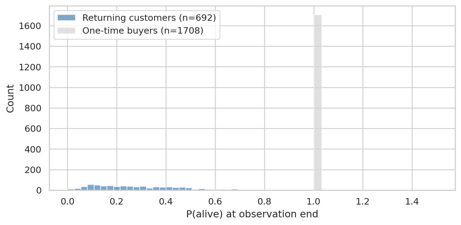
#| label: fig-p-alive
#| fig-cap: "Distribution of P(alive). One-time buyers concentrate near the population baseline; repeat customers split between still-engaged (right) and lapsed (left tail)."
fig, ax = plt.subplots(figsize=(8, 4))
returning = summary[(summary["frequency"] >= 1) & (summary["monetary_value"] > 0)]
one_time = summary[summary["frequency"] == 0]
ax.hist(returning["p_alive"], bins=30, alpha=0.7, color="steelblue", label=f"Returning customers (n={len(returning)})")
ax.hist(one_time["p_alive"], bins=30, alpha=0.7, color="lightgrey", label=f"One-time buyers (n={len(one_time)})")
ax.set_xlabel("P(alive) at observation end")
ax.set_ylabel("Count")
ax.legend()
plt.tight_layout()
plt.show()
```
The split is exactly what the model is designed to surface: customers who bought once recently (high *T* unobserved, no repeats yet) get a baseline P(alive) tied to the population; customers with multiple recent purchases get high P(alive); customers who used to buy but went quiet get low P(alive).
## Add monetary — Gamma-Gamma
Gamma-Gamma estimates expected per-transaction value. It can only be fit on customers with **at least one repeat purchase** (otherwise we have no within-customer monetary spread). Two best-practice precautions before fitting:
1. **Drop non-positive monetary values.** Real retail data has refunds netting to ≤ 0; Gamma-Gamma is defined on the positive reals.
2. **Trim the top-1% extreme values.** A handful of very-high-basket customers (think bulk order, contract sale, or data entry typo) can pull the Gamma fit and inflate population CLV. Industry practice is to winsorise or trim before fitting; we trim at the 99th percentile and report how many customers were affected.
```{python}
#| label: fit-gamma-gamma
returning = summary[(summary["frequency"] >= 1) & (summary["monetary_value"] > 0)].copy()

# Trim top-1% monetary outliers (capped at P99) — the Gamma-Gamma fit is
# sensitive to extreme high values otherwise.
p99 = returning["monetary_value"].quantile(0.99)
n_above = int((returning["monetary_value"] > p99).sum())
print(f"Monetary value trim: {n_above} customers (top 1%) above €{p99:,.0f} "
      f"capped to that level before Gamma-Gamma fit.")
returning["monetary_value"] = returning["monetary_value"].clip(upper=p99)

ggf = GammaGammaFitter(penalizer_coef=0.01)
ggf.fit(returning["frequency"], returning["monetary_value"])
ggf.summary.round(3)
```
```{python}
#| label: predicted-monetary
returning["exp_avg_value"] = ggf.conditional_expected_average_profit(
    returning["frequency"], returning["monetary_value"]
)
returning[["frequency", "monetary_value", "exp_avg_value"]].describe().round(2)
```
`exp_avg_value` shrinks toward the population mean for customers with few transactions (we have less evidence about their personal "true" value) and approaches the customer's own historical mean as their frequency grows. This Bayesian shrinkage is one of the model's strengths.
## Putting it together — 12-month CLV
```{python}
#| label: clv
HORIZON_MONTHS = 12
DISCOUNT_RATE  = 0.01  # monthly

returning["clv_12m"] = ggf.customer_lifetime_value(
    bgf,
    returning["frequency"],
    returning["recency"],
    returning["T"],
    returning["monetary_value"],
    time=HORIZON_MONTHS,
    discount_rate=DISCOUNT_RATE,
    freq="D",
)

returning[["frequency", "recency", "p_alive", "exp_avg_value", "clv_12m"]].describe().round(2)
```
```{python}
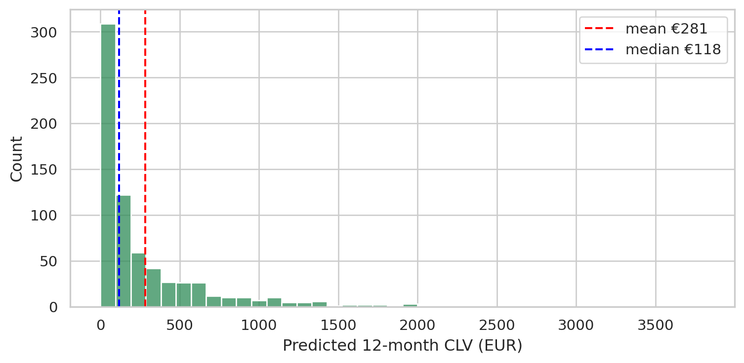
#| label: fig-clv-distribution
#| fig-cap: "12-month CLV distribution among returning customers. Long-tailed — most customers contribute modestly, a small head drives a disproportionate share of forecast revenue."
fig, ax = plt.subplots(figsize=(8, 4))
sns.histplot(returning["clv_12m"], bins=40, ax=ax, color="seagreen")
ax.axvline(returning["clv_12m"].mean(),   color="red",  ls="--", label=f"mean €{returning['clv_12m'].mean():.0f}")
ax.axvline(returning["clv_12m"].median(), color="blue", ls="--", label=f"median €{returning['clv_12m'].median():.0f}")
ax.set_xlabel("Predicted 12-month CLV (EUR)")
ax.legend()
plt.tight_layout()
plt.show()
```
### Pareto check — top 20% vs. rest
```{python}
#| label: pareto
returning_sorted = returning.sort_values("clv_12m", ascending=False)
total_clv = returning_sorted["clv_12m"].sum()
top_20_clv = returning_sorted["clv_12m"].iloc[: int(0.2 * len(returning_sorted))].sum()
print(f"Top 20% of returning customers account for {top_20_clv / total_clv:.1%} of forecast 12-month revenue.")
```
Concentrating retention spend on the top decile of forecast CLV is a much stronger lever than treating everyone equally.
```{python}
#| label: top-customers
returning_sorted.head(10)[
    ["frequency", "recency", "T", "monetary_value", "p_alive", "exp_avg_value", "clv_12m"]
].round(2)
```
## What this chapter buys you that RFM doesn't
The earlier RFM chapter clusters customers (or articles) by recency, frequency, monetary value into discrete tiers. It's interpretable but punchy: a customer in cluster 2 versus 3 is *different*, period.
BG/NBD + Gamma-Gamma gives **continuous, probabilistic, time-shifted** predictions:
- *Continuous*: every customer gets a real-valued expected purchase count and CLV, not a categorical tier
- *Probabilistic*: outputs come with implied uncertainty (the Gamma/Beta priors); cohorts of similar customers will differ in P(alive) and CLV reflecting available evidence
- *Time-shifted*: it forecasts *forward* over a chosen horizon, while RFM is purely a snapshot of the past
For decisions like "who do we send this win-back email to?" or "which customers should our retention team call?", the predicted P(alive) and CLV are directly actionable in a way RFM cluster IDs are not.
## Limitations
- **One-time buyers**: BG/NBD can score them (population-baseline P(alive) and expected purchases) but Gamma-Gamma cannot — they have no within-customer monetary spread. We treated them separately above.
- **Synthetic-data caveat**: this dataset was generated under BG/NBD-like assumptions, so the model fits cleanly. Real retail data has structure the model doesn't capture (seasonality, marketing pushes, life events). The output is still useful but holdout validation matters more.
- **Furniture is unusual**: customers buy infrequently. Models tuned on FMCG (groceries, toiletries) often need parameter tweaks for durable goods.