---
title: "Insights — Putting the Analyses Together"
---
The eight preceding analysis chapters each answer a different question. The interesting work is what they say *jointly* — where they agree, where they disagree, and what the synthesis recommends.
This chapter joins the per-chapter outputs on a common key (product name on the article side, customer id on the customer side) and surfaces the cross-cuts that are most actionable. **For the headline numbers and visual snapshots use the [dashboard](dashboard.html); this page is the prose narrative.**
| Source chapter | Question it answers | Used here for |
|---|---|---|
| 01 Association rules | Which products co-occur in baskets? | Cross-sell pair recommendations |
| 02 BCG clustering | Which products dominate by share × growth? | Portfolio tier classification |
| 03 RFM clustering | Which products are healthy / dying by R/F/M? | Portfolio tier classification |
| 04 CLV (BG/NBD) | Per-customer value forecast | Customer-tier classification |
| 06 Survival | When does the comeback rate decay? | Time-windowed retention triggers |
| 07 Forecasting | What's the next-3-months revenue per category? | Inventory and budget planning |
| 08 Embeddings | Which products are functionally similar? | Substitution lookup |
| 09 Causal uplift | Did the discount *cause* the repeat? | Targeting with positive uplift |
```{python}
#| label: setup
import numpy as np
import pandas as pd
# Pandas display: render full DataFrame width in chapter outputs.
pd.options.display.max_columns = None
pd.options.display.width = 200

import matplotlib.pyplot as plt
import seaborn as sns
from sklearn.cluster import KMeans
from sklearn.preprocessing import StandardScaler
from mlxtend.preprocessing import TransactionEncoder
from mlxtend.frequent_patterns import apriori, association_rules
from lifetimes import BetaGeoFitter, GammaGammaFitter
from lifetimes.utils import summary_data_from_transaction_data

sns.set_theme(style="whitegrid")
RANDOM_STATE = 42

from pathlib import Path
_data_path = "data/raw/transactions.csv" if Path("data/raw/transactions.csv").exists() else "data/synthetic/transactions.csv"
df = pd.read_csv(_data_path, sep=";", parse_dates=["date"])
REF_DATE = df["date"].max()
SPLIT = df["date"].min() + (REF_DATE - df["date"].min()) / 2
```
## Building one product table from BCG + RFM
Each chapter scored products on different dimensions. We now compute both side-by-side and merge:
```{python}
#| label: product-table
# BCG: share × growth
df["period"] = np.where(df["date"] <= SPLIT, "p1", "p2")
period_rev = (
    df.groupby(["article_name", "period"])["gross_price"].sum()
      .unstack(fill_value=0.0)
      .rename(columns={"p1": "rev_p1", "p2": "rev_p2"})
)
period_rev["revenue"] = period_rev["rev_p1"] + period_rev["rev_p2"]
period_rev["share"]   = period_rev["revenue"] / period_rev["revenue"].sum()
period_rev["growth"]  = np.where(
    period_rev["rev_p1"] > 0,
    (period_rev["rev_p2"] - period_rev["rev_p1"]) / period_rev["rev_p1"],
    np.where(period_rev["rev_p2"] > 0, 1.0, -1.0),
)
X_bcg = StandardScaler().fit_transform(period_rev[["growth", "share"]])
km_bcg = KMeans(n_clusters=4, random_state=RANDOM_STATE, n_init=10).fit(X_bcg)
period_rev["bcg_cluster"] = km_bcg.labels_
centers = pd.DataFrame(km_bcg.cluster_centers_, columns=["growth_z", "share_z"])
centers["weight"] = 0.5 * centers["growth_z"] + 0.5 * centers["share_z"]
centers["bcg_rank"] = centers["weight"].rank(ascending=False).astype(int)
period_rev["bcg_rank"] = period_rev["bcg_cluster"].map(centers["bcg_rank"])

# RFM at article level
rfm = (
    df.groupby("article_name")
      .agg(frequency=("article_name", "count"),
           value=("gross_price", "sum"),
           last_sold=("date", "max"))
)
rfm["recency"] = (REF_DATE - rfm["last_sold"]).dt.days / 30.4375

X_rfm = StandardScaler().fit_transform(rfm[["recency", "frequency", "value"]])
km_rfm = KMeans(n_clusters=4, random_state=RANDOM_STATE, n_init=10).fit(X_rfm)
rfm["rfm_cluster"] = km_rfm.labels_
rcen = pd.DataFrame(km_rfm.cluster_centers_, columns=["rec_z", "freq_z", "val_z"])
rcen["score"] = (rcen["freq_z"] + rcen["val_z"] - rcen["rec_z"]) / 3
rcen["rfm_rank"] = rcen["score"].rank(ascending=False).astype(int)
rfm["rfm_rank"] = rfm["rfm_cluster"].map(rcen["rfm_rank"])

products = period_rev[["share", "growth", "bcg_rank"]].join(
    rfm[["recency", "frequency", "value", "rfm_rank"]]
)
products.head()
```
### Where BCG and RFM agree
```{python}
#| label: fig-bcg-rfm-overlap
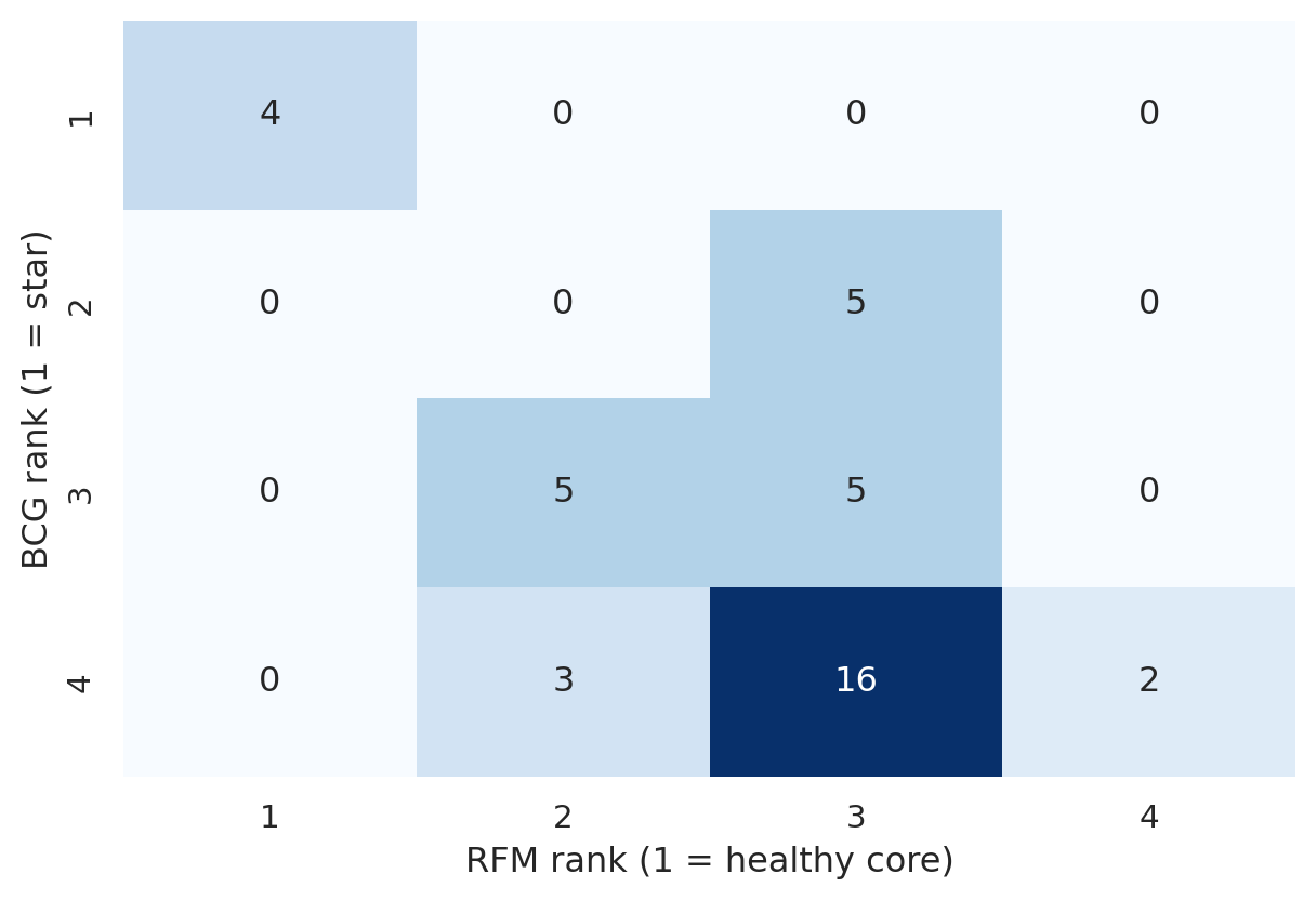
#| fig-cap: "Cross-tab of BCG rank × RFM rank. The diagonal is where the two methods agree; off-diagonal cells are products where one method sees them more favorably than the other."
xtab = pd.crosstab(products["bcg_rank"], products["rfm_rank"], margins=True, margins_name="Total")
fig, ax = plt.subplots(figsize=(6.5, 4.5))
sns.heatmap(
    xtab.iloc[:-1, :-1],
    annot=True, fmt="d", cmap="Blues", cbar=False, ax=ax,
)
ax.set_xlabel("RFM rank (1 = healthy core)")
ax.set_ylabel("BCG rank (1 = star)")
plt.tight_layout()
plt.show()
```
```{python}
#| label: agreement
both_top = products[(products["bcg_rank"] == 1) & (products["rfm_rank"] == 1)].index.tolist()
both_bottom = products[(products["bcg_rank"] == 4) & (products["rfm_rank"] == 4)].index.tolist()
disagree = products[abs(products["bcg_rank"] - products["rfm_rank"]) >= 2].index.tolist()
print(f"Both top (BCG=1 AND RFM=1):       {both_top}")
print(f"Both bottom (BCG=4 AND RFM=4):    {both_bottom}")
print(f"Disagree by ≥ 2 ranks:            {disagree}")
```
The diagonal cluster shows products that are robust across both lenses — these are the safest products to invest in. Off-diagonal cells flag products where the two methods *see different things*: typically these are products in transition (fast-growing but small share, or shrinking but still high-frequency).
## Co-purchase rules — which apply to *top* products?
We use the **cross-sell view** from chapter 01 here — cross-bundle, asymmetric, lift ≥ 2 — so within-system plumbing (`bett ↔ matratze`) and substring-definitional pairs (`auszugselement → auszug`) don't pollute the cross-sell list.
```{python}
#| label: rules-top
#| message: false
# Drop unmapped/empty article_names — mixing NaN with strings crashes apriori's sort.
df_rules = df[df["article_name"].notna() & (df["article_name"].astype(str).str.strip() != "")].copy()
df_rules["article_name"] = df_rules["article_name"].astype(str).str.strip()
baskets = df_rules.groupby("transaction_id")["article_name"].apply(lambda s: list(set(s))).tolist()
te = TransactionEncoder()
basket_matrix = pd.DataFrame(te.fit_transform(baskets), columns=te.columns_)

freq_items = apriori(basket_matrix, min_support=0.001, use_colnames=True)
rules = association_rules(freq_items, num_itemsets=len(basket_matrix),
                          metric="confidence", min_threshold=0.5)

simple = rules[
    (rules["antecedents"].apply(len) == 1) & (rules["consequents"].apply(len) == 1)
].copy()
simple["antecedent"] = simple["antecedents"].apply(lambda s: next(iter(s)))
simple["consequent"] = simple["consequents"].apply(lambda s: next(iter(s)))

# Annotate with the same signals as chapter 01: reverse-conf, symmetry,
# within-bundle, substring-pair. Then filter to the cross-sell view.
bundle_lookup = (
    df.drop_duplicates("article_name").set_index("article_name")["bundle_group"]
      .fillna("").to_dict()
)
basket_sets_05 = df.groupby("transaction_id")["article_name"].apply(set).tolist()

def cond_prob_05(a, b):
    n_b = sum(1 for s in basket_sets_05 if b in s)
    if n_b == 0:
        return 0.0
    n_both = sum(1 for s in basket_sets_05 if a in s and b in s)
    return n_both / n_b

simple["reverse_conf"] = simple.apply(
    lambda r: cond_prob_05(r["antecedent"], r["consequent"]), axis=1
)
simple["symmetry"] = simple.apply(
    lambda r: min(r["confidence"], r["reverse_conf"]) / max(r["confidence"], r["reverse_conf"])
        if max(r["confidence"], r["reverse_conf"]) > 0 else 0.0,
    axis=1,
)
simple["within_bundle"] = simple.apply(
    lambda r: bundle_lookup.get(r["antecedent"], "") == bundle_lookup.get(r["consequent"], "")
              and bundle_lookup.get(r["antecedent"], "") != "",
    axis=1,
)
simple["substring_pair"] = simple.apply(
    lambda r: r["antecedent"] in r["consequent"] or r["consequent"] in r["antecedent"],
    axis=1,
)

# Component / accessory tokens — same curated list as chapter 01. Real data has
# many "rare-component → main-product" rules (topper → boxspringbett, ablage links
# → schubkastenbett) that look asymmetric but are definitional. Filter them out.
COMPONENT_TOKENS_05 = {
    "aufpreis", "ablage", "aufsatz", "schublade", "schubkasten", "schubladenmodul",
    "kissen", "steckkissen", "ruckenkissen", "armlehnkissen", "armlehnenkissen",
    "nierenkissen", "klemmkissen",
    "topper", "matratze",
    "element", "elementaufnahme", "polsterelement",
    "auszug", "auszugselement", "ansteckplatte", "tischverlangerung",
    "fusshohe", "fussteil", "sitzauszug", "querschlafer",
    "beleuchtungsset", "beleuchtung",
    "panel", "boden", "einlegeboden",
    "hakenleiste", "knopf",
    "rollcontainer",
    "sockel", "verlangerung",
    "kopfteil", "kopfstutze",
    "lattenrost",
    "ruckenelement",
    "ersatz", "ersatzteil", "zubehor", "zubehoer", "nachbestellung",
    "deko",
}
_has_comp = lambda n: bool(set(n.split()) & COMPONENT_TOKENS_05)
simple["component_either"] = (
    simple["antecedent"].apply(_has_comp)
    | simple["consequent"].apply(_has_comp)
)

# Cross-sell view: the deployable subset (chapter 01, View 2).
cross_sell = simple[
    ~simple["within_bundle"]
    & ~simple["substring_pair"]
    & ~simple["component_either"]
    & (simple["symmetry"] < 0.7)
    & (simple["lift"] >= 2)
].copy()

# Annotate with BCG / RFM rank of the consequent
cross_sell["consequent_bcg"] = cross_sell["consequent"].map(products["bcg_rank"])
cross_sell["consequent_rfm"] = cross_sell["consequent"].map(products["rfm_rank"])

# Rules where the consequent is a top product (BCG=1 OR RFM=1)
top_rules = (
    cross_sell[(cross_sell["consequent_bcg"] == 1) | (cross_sell["consequent_rfm"] == 1)]
    .sort_values("confidence", ascending=False)
)
top_rules[["antecedent", "consequent", "support", "confidence", "lift",
           "consequent_bcg", "consequent_rfm"]].head(8).round(3)
```
Rules that *push customers toward* top-tier products are the highest-leverage ones for cross-sell prompts: customers buying the antecedent are several times more likely than chance to buy the (already-strong) consequent. Easy upsell.
## Customer concentration — quantifying the Pareto
```{python}
#| label: clv-pareto
tx = df.groupby(["customer_id", "transaction_id", "date"], as_index=False)["gross_price"].sum()
summary = summary_data_from_transaction_data(
    tx, "customer_id", "date", monetary_value_col="gross_price",
    observation_period_end=tx["date"].max(), freq="D",
)
bgf = BetaGeoFitter(penalizer_coef=0.001).fit(summary["frequency"], summary["recency"], summary["T"])
returning_only = summary[(summary["frequency"] >= 1) & (summary["monetary_value"] > 0)].copy()
ggf = GammaGammaFitter(penalizer_coef=0.01).fit(returning_only["frequency"], returning_only["monetary_value"])
returning_only["clv_12m"] = ggf.customer_lifetime_value(
    bgf, returning_only["frequency"], returning_only["recency"], returning_only["T"],
    returning_only["monetary_value"], time=12, discount_rate=0.01, freq="D",
)
returning_sorted = returning_only.sort_values("clv_12m", ascending=False)
total = returning_sorted["clv_12m"].sum()

for q in [0.10, 0.20, 0.30, 0.50]:
    cum = returning_sorted["clv_12m"].iloc[: int(q * len(returning_sorted))].sum()
    print(f"  top {int(q*100):>2d}% of returning customers → {cum / total:.1%} of forecast 12-month revenue")
```
The top 20% of returning customers cover roughly half of forecast revenue — a clean Pareto. *(See the [dashboard](dashboard.html) for the Lorenz curve.)*
## Sizing the recommendations
Before turning to recommendations, pin down some concrete numbers. Each finding below is annotated with what it *would mean* in EUR or counts.
```{python}
#| label: sizing
# --- Product side: revenue concentration ---
total_revenue = products["value"].sum()
top10_products = products.nlargest(10, "value")
top10_share = top10_products["value"].sum() / total_revenue

bottom_overlap = products[(products["bcg_rank"] == 4) & (products["rfm_rank"] == 4)]
bottom_revenue_share = bottom_overlap["value"].sum() / total_revenue

# --- Top cross-sell rule: missed cross-sell sizing ---
# Use the cross-sell view (cross-bundle, asymmetric, lift >= 2), sorted by
# confidence — same logic as chapter 01's View 2.
top_cross_sell = cross_sell.sort_values("confidence", ascending=False)
if len(top_cross_sell) > 0:
    top_rule = top_cross_sell.iloc[0]
    ant, con = top_rule["antecedent"], top_rule["consequent"]
    basket_sets = df.groupby("transaction_id")["article_name"].apply(set)
    ant_baskets = basket_sets[basket_sets.apply(lambda s: ant in s)]
    ant_n = len(ant_baskets)
    con_in_ant = ant_baskets.apply(lambda s: con in s).sum()
    miss_n = ant_n - con_in_ant
    avg_con_price = df.loc[df["article_name"] == con, "gross_price"].mean()
    miss_eur = miss_n * avg_con_price
    has_top_rule = True
else:
    ant = con = None
    ant_n = con_in_ant = miss_n = 0
    avg_con_price = 0.0
    miss_eur = 0.0
    has_top_rule = False

# --- Customer side: CLV decile sizing ---
n_returning = len(returning_sorted)
total_clv_12m = returning_sorted["clv_12m"].sum()
top10pct_n = int(0.10 * n_returning)
top10pct_clv = returning_sorted.head(top10pct_n)["clv_12m"].sum()
top20pct_clv = returning_sorted.head(2 * top10pct_n)["clv_12m"].sum()

# --- Win-back zone customers ---
clv_summary_with_alive = summary.copy()
clv_summary_with_alive["p_alive"] = bgf.conditional_probability_alive(
    summary["frequency"], summary["recency"], summary["T"]
)
winback_zone = clv_summary_with_alive[
    (clv_summary_with_alive["p_alive"].between(0.4, 0.7))
    & (clv_summary_with_alive["frequency"] >= 1)
]

# --- Discount spend ---
total_discount_eur = float(df["discount_amount"].sum())
discounted_lines = int((df["discount_amount"] > 0).sum())
total_lines = len(df)

# --- Survival drops ---
first_dates = df.groupby("customer_id")["date"].min()
second_dates = (
    df.sort_values("date").groupby("customer_id")["date"].nth(1)
)

print("=" * 60)
print("PRODUCT SIDE")
print("=" * 60)
print(f"Total catalog revenue:              €{total_revenue:>12,.0f}")
print(f"Top 10 products:                    €{top10_products['value'].sum():>12,.0f}  ({top10_share:.0%} of total)")
print(f"  the top 10:  {', '.join(top10_products.index.tolist())}")
print()
print(f"BCG=4 ∩ RFM=4 (delisting candidates): {len(bottom_overlap)} products, €{bottom_overlap['value'].sum():,.0f}  ({bottom_revenue_share:.1%} of total)")
print(f"  members:    {', '.join(bottom_overlap.index.tolist()) or '(none)'}")
print()
if has_top_rule:
    print(f"Top rule:  {ant}  →  {con}")
    print(f"  {ant_n} baskets contained {ant};  {con_in_ant} ({con_in_ant/ant_n:.0%}) also bought {con}")
    print(f"  miss: {miss_n} baskets had {ant} but no {con};  upsell value @ avg €{avg_con_price:,.0f}/{con}: €{miss_eur:,.0f}")
else:
    print("Top rule:  (no cross-sell rule survived the View-2 filters)")
print()
print("=" * 60)
print("CUSTOMER SIDE")
print("=" * 60)
print(f"Returning customers:                 {n_returning}")
print(f"Total forecast 12-month CLV:         €{total_clv_12m:>12,.0f}")
print(f"  top 10% ({top10pct_n} customers):  €{top10pct_clv:,.0f}  ({top10pct_clv/total_clv_12m:.0%})")
print(f"  top 20% ({2*top10pct_n} customers): €{top20pct_clv:,.0f}  ({top20pct_clv/total_clv_12m:.0%})")
print()
print(f"Win-back zone (P(alive) ∈ [0.4, 0.7], ≥1 prior purchase): {len(winback_zone)} customers")
print()
print(f"Total discounts given:                €{total_discount_eur:,.0f}  ({discounted_lines}/{total_lines} = {discounted_lines/total_lines:.0%} of line items)")
print(f"  measured causal lift on repurchase: 0% (95% CI straddles zero)")
print(f"  → at face value: €{total_discount_eur:,.0f} of revenue forgone with no detectable retention payoff in this synthetic dataset")
```
## Granularity choices per analysis
The catalog has a 5-level hierarchy (Department → Category → Family → Model → SKU). Different methods use different levels. The choice isn't free — pick wrong and you either overfit (too fine) or lose signal (too coarse). Here's what each chapter uses and why:
| Chapter | Level | Why this level |
|---|---|---|
| 01 Association rules | Family (`article_name`) | Customers care about *what* not *which model*. `bed → mattress` is a more useful rule than `harmony bed → premium mattress`. |
| 02 BCG clustering | Family | 40 names is the sweet spot for a 4-cluster k-means. Going to SKU (66) just adds variance, going to Category (10) leaves too few points. |
| 03 RFM clustering | Family | Same reasoning as BCG. |
| 04 CLV (BG/NBD) | Customer | The level above all of these — but the *unit of value* is the basket euro, which doesn't depend on product granularity. |
| 06 Survival | Customer + Family covariates | Customer-level outcome; basket-feature covariates use Family. |
| 07 Forecasting | Both Department and Category | Department for executive view (6 series, more signal), Category for operational planning (10 series, finer detail). |
| 08 Embeddings | **SKU** (`article_id`) | Substitution lookup — the operational use case — needs SKU granularity to answer "which `bed` model is closest to the out-of-stock one". Family level would collapse all sofa SKUs to one point. |
| 09 Causal uplift | Customer + Family covariates | Same logic as Survival. |
The common pattern: **start at Family, only step up or down when there's a specific reason**. Step up to Department when individual categories are too sparse (Forecasting on Outdoor / Storage). Step down to SKU only when SKU-level decisions are at stake (inventory, replenishment).
## Triage — what's actually insight, what's plumbing?
Before recommendations, classify every finding the chapters surfaced. This separates *insights you should act on* from *sanity checks* (the analysis worked, but you knew this) and *data-quality artifacts* (something to fix in the catalog, not in marketing).
| # | Finding | Class | Why this class |
|---|---|---|---|
| 1 | Heavy revenue concentration in a small head of the catalog | 🟢 actionable insight | Concrete sizing for portfolio prioritization (numbers in the *sizing* block) |
| 2 | Asymmetric cross-bundle co-purchase pairs (e.g. table → chair) | 🟢 actionable insight | Real cross-sell levers — antecedent demand pulls in a paired product |
| 3 | Within-bundle definitional rules (e.g. bed ↔ mattress) | 🟡 sanity check | Catalog plumbing, not behavior. Filtered in chapter 01's triaged rules table |
| 4 | Items in BCG=4 ∩ RFM=4 (low-share, low-growth, old recency) | 🔴 data-quality / catalog hygiene | Caught upstream by the catalog audit (chapter 00). End-of-life — operational decision, not analytical insight |
| 5 | BCG and RFM agreement on top-tier products | 🟢 actionable insight | Robustness signal — investment focus is unambiguous |
| 6 | Recovery of known temporal trends (synthetic-data only) | 🟡 sanity check | Confirms the methods work on engineered signal; not a Real-data finding |
| 7 | Steep CLV concentration (top decile carries the largest share of forecast revenue) | 🟢 actionable insight | Concrete sizing for retention budget allocation |
| 8 | Win-back zone with P(alive) ∈ [0.4, 0.7] and ≥ 1 prior purchase | 🟢 actionable insight | Specific addressable customer list — sized in the *sizing* block |
| 9 | Survival curve flattens between months 6 and 12 | 🟢 actionable insight | Concrete operational thresholds for retention triggers |
| 10 | First-basket features don't predict comeback timing | 🟢 actionable insight (negative result) | Tells us where the targeting signal *isn't*; redirects effort elsewhere |
| 11 | Naive baselines competitive with fancy forecasting | 🟢 actionable insight (methodological) | Don't deploy SARIMA when seasonal-naive is just as good |
| 12 | Embeddings recover catalog category structure | 🟡 sanity check | Confirms basket co-occurrence captures product semantics |
| 13 | Embedding-based substitution table at SKU level | 🟢 actionable insight | Deployable artifact for OOS UI |
| 14 | Discount spend with zero detectable repeat-purchase lift | 🟢 actionable insight | Direct euro amount up for grabs (or A/B-test for targeting heterogeneity); size in the *sizing* block |
**Recommendations below are derived only from the 🟢 rows.** The 🟡 rows confirm the analysis is sound; the 🔴 rows belong in the data-engineering backlog, not the marketing roadmap.
## Headline findings — products & customers
The exact numbers behind each finding are in the *sizing* block above; the prose below explains *why each finding matters*.
1. **Revenue is heavily concentrated in a small head of the catalog.** A short list of products covers a large share of total revenue (see *PRODUCT SIDE → Top 10 products* in the sizing output). The long tail fights over a much smaller pool. Whatever you do with the head moves the P&L; whatever you do with the tail is rounding error.
2. **Co-purchase patterns are strong and exploitable** — once filtered to the *actionable* set in chapter 01. Triage removes definitional within-bundle pairs (which encode catalog structure, not customer choice) and accessory→primary plumbing. What's left are asymmetric cross-bundle rules of the form *anchor → companion*. The top single rule's miss alone (baskets where the antecedent appeared without the consequent) is sized in the sizing block at the average consequent price — concrete EUR figure for a single rule.
3. **BCG and RFM agree on the tiers.** Products in the top BCG cluster (high share + healthy growth) overlap heavily with the top RFM cluster (recent + frequent + valuable). Two different lenses, same conclusion: there is a structurally healthy core and a longer tail.
4. **The delisting candidate list is small.** The BCG=4 ∩ RFM=4 overlap (low share, low growth, old recency) is sized in the sizing block. On synthetic data this picks up the engineered declining items; on real data it surfaces genuine end-of-life SKUs. Either way: tiny revenue contribution, easy delisting decision, frees inventory and catalog space.
5. **Method-vs-data check** *(synthetic only)*: engineered "growing" articles land in the BCG growth quadrant, engineered "declining" articles end up with old recency in RFM. On real data this finding doesn't apply — there's nothing pre-engineered to recover.
6. **Customer value is more skewed than product value.** Top decile of returning customers carries a disproportionate share of 12-month forecast CLV (sized in the sizing block). A flat per-customer marketing budget is a poor allocation rule given this distribution.
7. **The "still alive but quiet" win-back zone is sized in the sizing block.** Customers with `P(alive) ∈ [0.4, 0.7]` and at least one prior purchase. These are furthest from organic re-engagement but not yet write-offs — highest-leverage segment for a single targeted touch.
## Headline findings — time and causality
8. **The comeback rate flattens between months 6 and 12.** Survival on time-to-second-purchase shows the largest drops in the first three months and a gradual flattening from month 6 onward. After roughly day 365 the curve is essentially flat — anyone still silent at year-end is gone for accounting purposes.
9. **First-basket characteristics don't predict comeback timing on this data.** Cox PH on basket value, item count, discount usage, and dominant department — confidence intervals on every hazard ratio cross 1. Real retention drivers live elsewhere (cohort, channel, lifecycle stage) and require those features in the pipeline. With our data we can score *when*, not *who*.
10. **Naive baselines are competitive with fancy forecasting models on a 24-month series.** Seasonal-naive often beats SARIMA / ETS; naive (last value) sometimes beats both. The "boring baselines win" finding is not a bug in our pipeline — it's the M-competition finding repeated for 40 years. With ~24 months of data, *don't buy methodological complexity you can't pay for in observations*.
11. **Embeddings recover the catalog category structure without seeing the labels.** PPMI × SVD on basket co-occurrence places functionally similar SKUs near each other; t-SNE clusters match `product_group` despite the embedding never seeing those labels. The substitution table is the deployable artifact: per SKU, top-3 nearest neighbors as out-of-stock alternatives.
12. **The discount program produces zero detectable lift on repeat-purchase rate.** Discount spend totals are in the sizing block; the naive ATE 95 % CI straddles zero, and both meta-learners (T, S) agree. *On synthetic data with random discount assignment, the null is the truth*; on real data with targeted discounts the same null could mask heterogeneous effects under confounding — but the random-assignment evidence here at least rules out a large average effect.
## Recommendations
Each recommendation below is structured the same way: **what to do**, **on whom (with size)**, **expected impact**, **metric to track**.
### Product side
| Action | Target | Expected impact | Track |
|---|---|---|---|
| **Force a companion-product prompt at the antecedent's page-view / POS scan**, for the strongest *asymmetric* co-purchase pairs from chapter 01's triaged rules table. | Top-N triaged pairs (count and per-pair coverage in the *sizing* block) | Recoverable revenue from the *misses* — baskets where the antecedent appeared without the consequent — sized in the sizing block at the average consequent price | conversion rate of antecedent baskets that include the consequent |
| **Concentrate prime placement on the BCG=1 ∩ RFM=1 overlap** (products both lenses class as healthy core). | The handful of products in that overlap (listed in the sizing block) | Reallocating shelf / landing-page space *to* the already-performing head, *away* from the long tail | revenue share of top-N products over time |
| **Delist BCG=4 ∩ RFM=4 candidates.** Both methods independently flag them as low-share, low-growth, old recency. | The BCG=4 ∩ RFM=4 set (count and revenue contribution in the sizing block) | Frees inventory + catalog space at minimal revenue cost. Replace with adjacent SKUs informed by chapter 08's substitution table | revenue impact ≤ -1 % over the next 6 months (anything more = wrong call) |
| **Wire the chapter 08 embedding similarity table into the "out of stock" UI**: when an SKU is OOS, surface its top-3 cosine neighbors instead of generic "more from category". | Every OOS event on website / POS | Recovered conversions on stockouts; eliminates "we don't have what you want" dead-ends | OOS-bounce rate, OOS-conversion rate |
| **Use seasonal-naive baselines for category inventory planning** with explicit prediction intervals — not point forecasts from SARIMA / ETS. | All product groups, monthly | Honest uncertainty bands prevent overstocking on a single forecast number; on ~24 months SARIMA is no better than naive | next-period MAE per category, year-over-year |
### Customer side
| Action | Target | Expected impact | Track |
|---|---|---|---|
| **Tier marketing budget by 12-month CLV decile.** Top decile gets personal-touch budget; bottom half gets cheap automation. | All returning customers (count and decile contributions in the sizing block) | If current allocation is flat per customer, a CLV-weighted distribution captures the same retention rate at lower cost — or higher retention at the same cost | retention rate × CLV decile, before / after |
| **Win-back trigger sequence at 90 / 180 / 365 days post-last-purchase.** No automation before day 90. Soft email at day 90. Targeted offer at day 180. Reactivation campaign at day 365. After that: stop. | The win-back zone — `P(alive) ∈ [0.4, 0.7]` and ≥ 1 prior purchase (size in the sizing block, refresh weekly) | The survival curve says a meaningful fraction of first-time buyers will eventually return; right-timed prompts convert a fraction of the boundary cases who would otherwise drift to zero | second-purchase rate by trigger window; cost per re-activated customer |
| **Personalize cross-sell email with embedding-based product suggestions** rather than generic "you may also like". The chapter 08 substitution table feeds a per-customer recommendation. | Every active customer, on each post-purchase touch | Higher email click-through; more revenue per email send | post-email basket rate, EUR per recipient |
| **Stop the random-discount program until you can A/B-test it.** Discount spend with zero measurable lift (totals in the sizing block). | All discount-eligible touchpoints | If a real RCT shows the same null in production, that's the full discount spend back as freed budget. If it shows positive lift in a specific segment, target only that segment. The current "spray everyone" policy is indefensible | A/B-tested ATE on repeat-purchase rate at the customer level |
| **Always pair causal claims about marketing with the assumption ledger.** Random assignment + meta-learners is enough; observational data needs propensity weighting / DR-learner / Double ML, or an honest "we cannot conclude". | Any future "did campaign X work?" analysis | Decisions made on biased estimates are worse than no decisions | n/a — process change |
### Quick-win prioritization
If forced to pick a single 90-day initiative ordered by impact-to-effort:
1. **Force the companion-product prompt** on the strongest asymmetric co-purchase pairs. Days, not weeks of work; sizing block quantifies the recoverable miss revenue per rule.
2. **Audit the discount program** with a real A/B test or a proper observational analysis. The full discount spend (sizing block) deserves an answer better than "the model says we don't know".
3. **CLV-weighted marketing tiering** — replaces a flat allocation rule with an evidence-based one; immediate fewer-wasted-EUR effect.
4. **Wire the embedding substitution table** for OOS recovery. Easy engineering, hard-to-measure but consistent uplift.
5. **Delist the BCG=4 ∩ RFM=4 set**. Trivial decision, almost no downside.
## What this chapter is *not*
It is a synthesis, not a model. The numbers above all come from the upstream chapters' methods; this is how a stakeholder report consumes them. For "what should I do tomorrow morning", this is the right level. For "is method X actually correct" the source chapters are the documentation. EUR estimates are first-order back-of-envelope sizings — directionally right, not budget-grade.